1. The metric-based framework

The goal-oriented mesh adaptation functionality in Goalie is designed such that it is agnostic of the specific method used to modify the mesh. However, to give a concrete example, this section describes the metric-based mesh adaptation framework. Integration of this adaptation approach into the Firedrake finite element library is currently underway.

1.1. Metric spaces

The metric-based framework has its roots in Riemannian geometry - in particular, Riemannian metric spaces.

A metric space \((\mathcal V,\underline{\mathbf M})\) consists of a vector space \(\mathcal V\) and a metric \(\underline{\mathbf M}\) defined upon it. Under the assumption that \(\mathcal V=\mathbb R^n\) for some \(n\in\mathbb N\), \(\mathcal M\) can be represented as a real \(n\times n\) symmetric positive-definite (SPD) matrix. From the metric, we may deduce a distance function and various geometric quantities related to the metric space. The most well-known example of an \(n\)-dimensional metric space is Euclidean space, \(\mathbb E^n\). Euclidean space is \(\mathbb R^n\), with the \(n\)-dimensional identity matrix \(\underline{\mathbf I}\) as its metric. This gives rise to the well-known \(\ell_2\) distance function,

(1)\[d_2(\mathbf u,\mathbf v) :=\sqrt{\sum_{i=1}^n(v_i-u_i)^2} =\sqrt{(\mathbf{v}-\mathbf{u})^T\:\underline{\mathbf I}\:(\mathbf{v}-\mathbf{u})} =\sqrt{\vec{\mathbf{uv}}^T\:\underline{\mathbf M}\:\vec{\mathbf{uv}}},\]

where \(\vec{\mathbf{uv}}\) denotes the vector from \(\mathbf u=(u_1,\dots,u_n)\in\mathbb R^n\) to \(\mathbf v=(v_1,\dots,v_n)\in\mathbb R^n\).

The definition above assumes that the metric takes a fixed value. A Riemannian metric space, on the other hand, is defined point-wise on a domain \(\Omega\), such that its value is an \(n\times n\) SPD matrix at each point \(\mathbf x\in\Omega\). We use the notation \(\mathcal M=\{\underline{\mathbf M}(\mathbf x)\}_{\mathbf x\in\Omega}\) for the Riemannian metric. Throughout this documentation, the term metric should be understood as referring specifically to a Riemannian metric. The fact that a Riemannian metric can vary in space means that Riemannian metric spaces are warped, when viewed in Euclidean space. For example, think of the space-time continuum in General Relativity. This is probably the most famous example of a Riemannian metric space.

An example of a Riemannian metric space: the gravitational field of the Earth (source: Wikipedia).

Given a Riemannian metric \(\mathcal M=\{\underline{\mathbf M}(\mathbf x)\}_{\mathbf x\in\Omega}\), we can define distance in the associated space as above. However, since space is warped, we need to integrate along a curve, rather than a straight line. Given that \(\boldsymbol\gamma:[0,1]\rightarrow\mathbb R^n\) parametrises the curve from \(\mathbf u\in\Omega\) to \(\mathbf v\in\Omega\), the distance may be computed using the parametric integral

(2)\[d_{\mathcal M}(\mathbf u,\mathbf v) :=\int_0^1\sqrt{\vec{\mathbf{uv}}\:\underline{\mathbf M}(\boldsymbol\gamma(\xi))\:\vec{\mathbf{uv}}}\;\mathrm d\xi.\]

We define length in the metric space by

(3)\[\ell_{\mathcal M}(\vec{\mathbf{uv}}) :=d_{\mathcal M}(\mathbf u,\mathbf v).\]

As well as distances and lengths, it is also possible to define volume in Riemannian space. Given a subset \(K\subseteq\Omega\), its volume is given by

(4)\[\left|K\right|_{\mathcal M} :=\int_K\sqrt{\underline{\mathbf M}(\mathbf x)}\;\mathrm dx.\]

The concept of angle also carries over, amongst other things.

Metric fields should be defined in Firedrake using firedrake.meshadapt.RiemannianMetrics from instances of a Lagrange firedrake.functionspace.TensorFunctionSpace() of degree 1, i.e. a tensor space that is piecewise linear and continuous. The following example code snippet defines a uniform metric, for example:

from firedrake import *
from firedrake.meshadapt import RiemannianMetric
from goalie import *

mesh = UnitSquareMesh(10, 10)
P1_ten = TensorFunctionSpace(mesh, "CG", 1)
metric = RiemannianMetric(P1_ten)
metric.interpolate(as_matrix([[1, 0], [0, 1]))

1.2. Geometric interpretation

A convenient way of visualising a Riemannian metric field is using an ellipse (in 2D) or an ellipsoid (in 3D). As mentioned above, the metric takes the form of an SPD matrix \(\underline{\mathbf M}(\mathbf x)\) at each point in space, \(\mathbf x\in\Omega\). Since it is symmetric, this matrix has an orthogonal eigendecomposition,

(5)\[\underline{\mathbf M}(\mathbf x) =\underline{\mathbf V}(\mathbf x)\: \underline{\boldsymbol\Lambda}(\mathbf x)\: \underline{\mathbf V}(\mathbf x)^T,\]

where \(\underline{\mathbf V}(\mathbf x)=\begin{bmatrix}\mathbf v_1,\dots,\mathbf v_n\end{bmatrix}\) is its matrix of (orthonormal) eigenvectors and \(\underline{\boldsymbol\Lambda}(\mathbf x)=\mathrm{diag}(\lambda_1,\dots,\lambda_n)\) is its matrix of eigenvalues.

Viewed in Euclidean space (i.e. the physical space), a 2D metric can be represented by an ellipse with \(i^{th}\) semi-axis taking the direction \(\mathbf e_i:=\mathbf v_i\) and having magnitude \(h_i:=1/\sqrt{\lambda_i}\). Viewed in the metric space (i.e. the control space), however, it is represented by a unit circle.

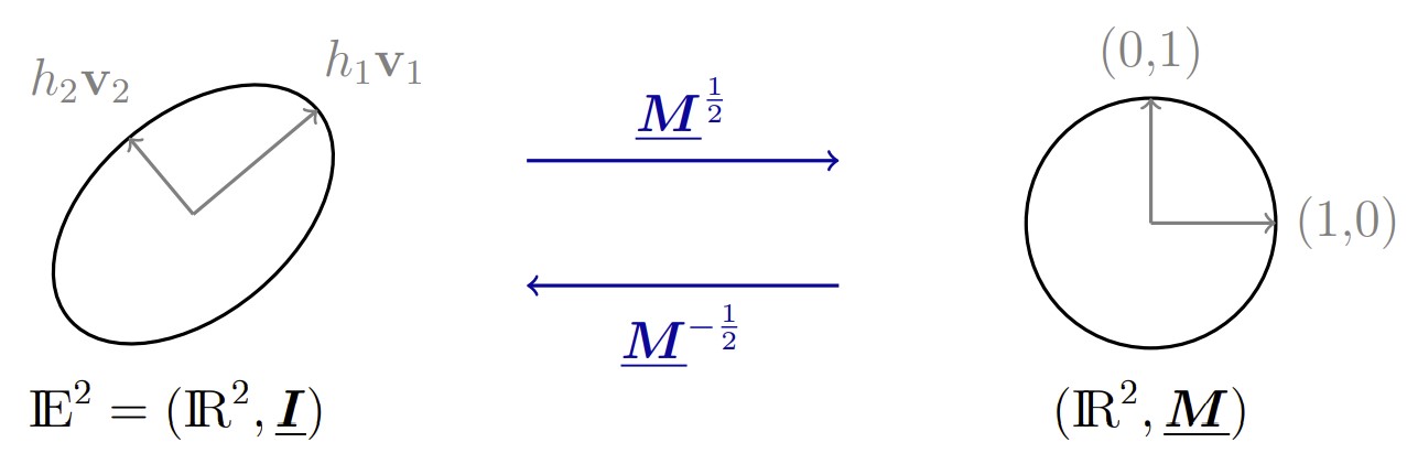
Representation of a 2D Riemannian metric as an ellipse. Image taken from [Wal21] with author’s permission.

Given a metric field, the eigendecomposition may be computed in Goalie using the function compute_eigendecomposition(). Similarly, given firedrake.function.Functions representing the eigenvectors and eigenvalues of a metric, it may be assembled using the function assemble_eigendecomposition().

The orthogonal eigendecomposition gives rise to another matrix decomposition, which is useful for understanding metric-based mesh adaptation. If we define metric density as the square root of the sum of the eigenvalues,

(6)\[\rho:=\sqrt{\prod_{i=1}^n\lambda_i},\]

and the \(i^{th}\) anisotropy quotient in terms of the metric magnitudes by

(7)\[r_i:=h_i^n\prod_{j=1}^n\frac1{h_j},\quad i=1,\dots,n,\]

then we arrive at the decomposition

(8)\[\underline{\mathbf M} =\rho^{\frac2n}\: \underline{\mathbf V}\: \mathrm{diag}\left(r_1^{-\frac2n},\dots,r_n^{-\frac2n}\right)\: \underline{\mathbf V}^T.\]

The reason that this formulation is useful is because it separates out information contained within the metric in terms of:

• sizes (the metric density);

• orientation (the eigenvectors);

• shape (the anisotropy quotients).

These are the three aspects of a mesh that metric-based mesh adaptation is able to control, whereas other mesh adaptation methods can only usually control element sizes.

The metric decomposition above can be computed in Goalie using the function density_and_quotients().

1.3. Continuous mesh analogy

The work of [LA11] established duality between the (inherently discrete) mesh and a (continuous) Riemannian metric field. Having a continuous representation for the mesh means that we are able to apply optimisation techniques that are designed for continuous problems.

An example of one of the correspondences is between metric complexity and mesh vertex count. Metric complexity is expressed using the formula

(9)\[\mathcal C(\mathcal M)=\int_\Omega\sqrt{\mathrm{det}(\mathcal M(\mathbf x)})\;\mathrm dx.\]

and can be interpreted as the volume of the spatial domain in metric space (recall the formula for volume in Riemannian space). Metric complexity may be computed in Firedrake using the method complexity(). The time-dependent extension of metric complexity,

(10)\[\mathcal C(\mathcal M)=\int_{\mathcal T}\int_\Omega\sqrt{\mathrm{det}(\mathcal M(\mathbf x,t)})\;\mathrm dx\;\mathrm dt\]

over a time interval \(\mathcal T\) is analogous to the total number of mesh vertices over all timesteps.

1.4. Metric-based mesh adaptation

The idea of metric-based mesh adaptation is to use a Riemannian metric space within the mesher. In doing so, we seek to modify the mesh so that in the metric space it is a so-called unit mesh. That is, all of its elements have unit edge length. For a 2D triangular mesh this means having a mesh comprised of equilateral elements with all sides being of length one. Making the elements consistent in metric space can be thought of in terms of equidistributing errors, which is one of the key ideas behind mesh adaptation in general.

In practice, it is not possible to tessellate space with regular elements. Therefore, we instead seek a quasi-unit mesh, whose elements are all “close to” unit, in some sense.

During the mesh adaptation process, the entities, nodal positions and/or connectivity are modified in order to move towards a quasi-unit mesh. The way that this is quantified in practice is using a quality function. For example, consider the 2D quality function

(11)\[Q_{\mathcal M} =\frac{\sqrt3}{12}\frac{\sum_{\boldsymbol\gamma\in\partial K}\ell_{\mathcal M}(\boldsymbol\gamma)^2}{| K|_{\mathcal M}},\]

where \(\boldsymbol\gamma\in\partial K\) indicates an edge from the edge set of element \(K\). It can be shown that \(Q_{\mathcal M}\) is minimised for an equilateral triangular element.

1.5. Operations on metrics

In order to use metrics to drive mesh adaptation algorithms for solving real problems, they must first be made relevant to the application. Metrics should be normalised in order to account for domain geometry, dimensional scales and other properties of the problem, such as the extent to which it is multi-scale.

In Firedrake, normalisation is performed by the method normalise() in the \(L^p\) sense:

(12)\[\mathcal M_{L^p}:= \mathcal C_T^{\frac2n} \:\left(\int_{\Omega}\mathrm{det}(\underline{\mathbf M})^{\frac p{2p+n}}\;\mathrm dx\right)^{-\frac2n} \:\mathrm{det}(\mathcal M)^{-\frac1{2p+n}} \:\mathcal M,\]

where \(\mathcal C_T\) is the target metric complexity (i.e. tolerated vertex count), \(n\) is the spatial dimension and \(p\in[1,\infty)\) is the order of the normalisation. Taking \(p=1\) implies a truly multi-scale metric and this becomes less so for higher orders. In the limit \(p\rightarrow\infty\) we obtain

(13)\[\mathcal M_{L^\infty}:= \left(\frac{\mathcal C_T}{\mathcal C(\mathcal M)}\right)^{\frac2n} \:\mathcal M.\]

For time-dependent problems, the normalisation formulation also includes integrals in time. Suppose \(\mathcal T\) is the time period of interest, \(\Delta t>0\) is the timestep and \(\mathcal C_T\) is now the target space-time complexity. Then the function space_time_normalise() computes

(14)\[\mathcal M_{L^p}:= \mathcal C_T^{\frac2n} \:\left(\int_{\mathcal T}\frac1{\Delta t}\int_\Omega\mathrm{det}(\underline{\mathbf M})^{\frac p{2p+n}}\;\mathrm dx\;\mathrm dt\right)^{-\frac2n} \:\mathrm{det}(\mathcal M)^{-\frac1{2p+n}} \:\mathcal M.\]

In many cases, it is convenient to be able to combine different metrics. For example, if we seek to adapt the mesh such that the value of two different error estimators are reduced. The simplest metric combination method from an algebraic perspective is the metric average:

(15)\[\tfrac12(\mathcal M_1 + \mathcal M_2),\]

for two metrics \(\mathcal M_1\) and \(\mathcal M_2\). Whilst mathematically simple, the geometric interpretation of taking the metric average is not immediately obvious. Metric intersection, on the other hand, is geometrically straight-forward, but non-trivial to write mathematically. The elliptic interpretation of two metrics is the largest ellipse which fits within the ellipses associtated with the two input metrics. As such, metric intersection yields a new metric whose complexity is greater than (or equal to) its parents’. This is not true for the metric average in general. See [PUDOG01] for details.

Intersection of two 2D Riemannian metrics, interpreted in terms of their elliptical representations. Image taken from [Wal21] with author’s permission.

Metric combination may be achieved in Goalie using the function combine_metrics(), which defaults to the metric average.

1.6. References

[LA11]

A Loseille and F Alauzet. Continuous mesh framework part I: well-posed continuous interpolation error. SIAM Journal on Numerical Analysis, 49(1):38–60, 2011. doi:10.1137/090754078.

[PUDOG01]

CC Pain, AP Umpleby, CRE De Oliveira, and AJH Goddard. Tetrahedral mesh optimisation and adaptivity for steady-state and transient finite element calculations. Computer Methods in Applied Mechanics and Engineering, 190(29-30):3771–3796, 2001. doi:10.1016/S0045-7825(00)00294-2.

[Wal21] (1,2)

JG Wallwork. Mesh adaptation and adjoint methods for finite element coastal ocean modelling. PhD thesis, Imperial College London, 2021. doi:10.25560/92820.