On-the-fly time-dependent mesh adaptation

In this demo we consider the two-dimensional version of the mesh adaptation experiment presented in []. The problem comprises a bubble of tracer concentration field advected by a time-varying flow. We will consider two different mesh adaptation strategies: the classical mesh adaptation algorithm, which adapts the mesh several times throughout the simulation based on the solution at the current time, and the metric advection algorithm, which advects the initial metric tensor along the flow in order to predict where to prescribe fine resolution in the future. Both algorithms are an example of on-the-fly time-dependent mesh adaptation algorithms, where the mesh is adapted before each subinterval of the simulation, as opposed to fixed-point iteration algorithms. Fixed-point iteration algorithms solve the equation of interest at each iteration, before adapting the mesh based on computed solutions at the end of each iteration. This clearly makes them effective at predicting where to prescribe fine resolution throughout the simulation, but implies substantial computational cost.

We begin by defining the advection problem. We consider the advection equation

\[\begin{split}\begin{array}{rl} \frac{\partial c}{\partial t} + \nabla\cdot(\mathbf{u}c)=0& \text{in}\:\Omega,\\ c=0 & \text{on}\:\partial\Omega,\\ c=c_0(x,y) & \text{at}\:t=0, \end{array},\end{split}\]

where \(c=c(x,y,t)\) is the sought tracer concentration, \(\mathbf{u}=\mathbf{u}(x,y,t)\) is the background velocity field, and \(\Omega=[0, 1]^2\) is the spatial domain of interest with boundary \(\partial\Omega\).

The background velocity field \(\mathbf{u}(x, y, t)\) is chosen to be periodic in time, and is given by

\[\mathbf{u}(x, y, t) := \left(2\sin^2(\pi x)\sin(2\pi y), -\sin(2\pi x)\sin^2(\pi y) \right) \cos(2\pi t/T),\]

where \(T\) is the period. At each timestep of the simulation we will update this field so we define a function that will return its vector expression.

from firedrake import *

T = 6.0


def velocity_expression(mesh, t):
    x, y = SpatialCoordinate(mesh)
    u_expr = as_vector(
        [
            2 * sin(pi * x) ** 2 * sin(2 * pi * y) * cos(2 * pi * t / T),
            -sin(2 * pi * x) * sin(pi * y) ** 2 * cos(2 * pi * t / T),
        ]
    )
    return u_expr

We proceed similarly with prescribing initial conditions. At \(t=0\), we initialise the tracer concentration \(c_0 = c(x, y, 0)\) to be \(1\) inside a circular region of radius \(r_0=0.15\) centred at \((x_0, y_0)=(0.5, 0.65)\) and \(0\) elsewhere in the domain. Note that such a discontinuous function will not be represented well on a coarse uniform mesh.

def get_initial_condition(mesh):
    x, y = SpatialCoordinate(mesh)
    ball_r, ball_x0, ball_y0 = 0.15, 0.5, 0.65
    r = sqrt(pow(x - ball_x0, 2) + pow(y - ball_y0, 2))
    c0 = Function(FunctionSpace(mesh, "CG", 1))
    c0.interpolate(conditional(r < ball_r, 1.0, 0.0))
    return c0

Now we are ready to solve the advection problem. Since we will solve the problem several times, we will wrap up the code in a function that we can easily call for each subinterval. The function takes the mesh over which to solve the problem, time interval \([t_{\text{start}}, t_{\text{end}}]\) over which to solve it, and the initial condition \(c_0 = c(x, y, t_{\text{start}})\). The function returns the solution \(c(x, y, t_{\text{end}})\).

Note that we include streamline upwind Petrov Galerkin (SUPG) stabilisation in the test function in order to ensure numerical stability.

def run_simulation(mesh, t_start, t_end, c0):
    Q = FunctionSpace(mesh, "CG", 1)
    V = VectorFunctionSpace(mesh, "CG", 1)
    R = FunctionSpace(mesh, "R", 0)

    c_ = Function(Q).project(c0)  # project initial condition onto the current mesh
    c = Function(Q)  # solution at current timestep

    u_ = Function(V).interpolate(velocity_expression(mesh, t_start))  # vel. at t_start
    u = Function(V)  # velocity field at current timestep

    # SUPG stabilisation
    D = Function(R).assign(0.1)  # diffusivity coefficient
    h = CellSize(mesh)  # mesh cell size
    U = sqrt(dot(u, u))  # velocity magnitude
    tau = 0.5 * h / U
    tau = min_value(tau, U * h / (6 * D))

    # Apply SUPG stabilisation to the test function
    phi = TestFunction(Q)
    phi += tau * dot(u, grad(phi))

    # Time-stepping parameters
    dt = Function(R).assign(0.01)  # timestep size
    theta = Function(R).assign(0.5)  # Crank-Nicolson implicitness

    # Variational form of the advection equation
    trial = TrialFunction(Q)
    a = inner(trial, phi) * dx + dt * theta * inner(dot(u, grad(trial)), phi) * dx
    L = inner(c_, phi) * dx - dt * (1 - theta) * inner(dot(u_, grad(c_)), phi) * dx

    # Define variational problem
    lvp = LinearVariationalProblem(a, L, c, bcs=DirichletBC(Q, 0.0, "on_boundary"))
    lvs = LinearVariationalSolver(lvp)

    # Integrate from t_start to t_end
    t = t_start + float(dt)
    while t < t_end + 0.5 * float(dt):
        # Update the background velocity field at the current timestep
        u.interpolate(velocity_expression(mesh, t))

        # Solve the advection equation
        lvs.solve()

        # Update the solution at the previous timestep
        c_.assign(c)
        u_.assign(u)
        t += float(dt)

    return c

Finally, we are ready to run the simulation. We will first solve the entire problem over two uniform meshes: one with 32 elements in each direction and another with 128 elements in each direction. Since the flow reverts to its initial state at time \(t=T/2\), we run the simulations over the interval \([0, T/2]\).

simulation_end_time = T / 2.0

mesh_coarse = UnitSquareMesh(32, 32)
c0_coarse = get_initial_condition(mesh_coarse)
c_coarse_final = run_simulation(mesh_coarse, 0.0, simulation_end_time, c0_coarse)

mesh_fine = UnitSquareMesh(128, 128)
c0_fine = get_initial_condition(mesh_fine)
c_fine_final = run_simulation(mesh_fine, 0.0, simulation_end_time, c0_fine)

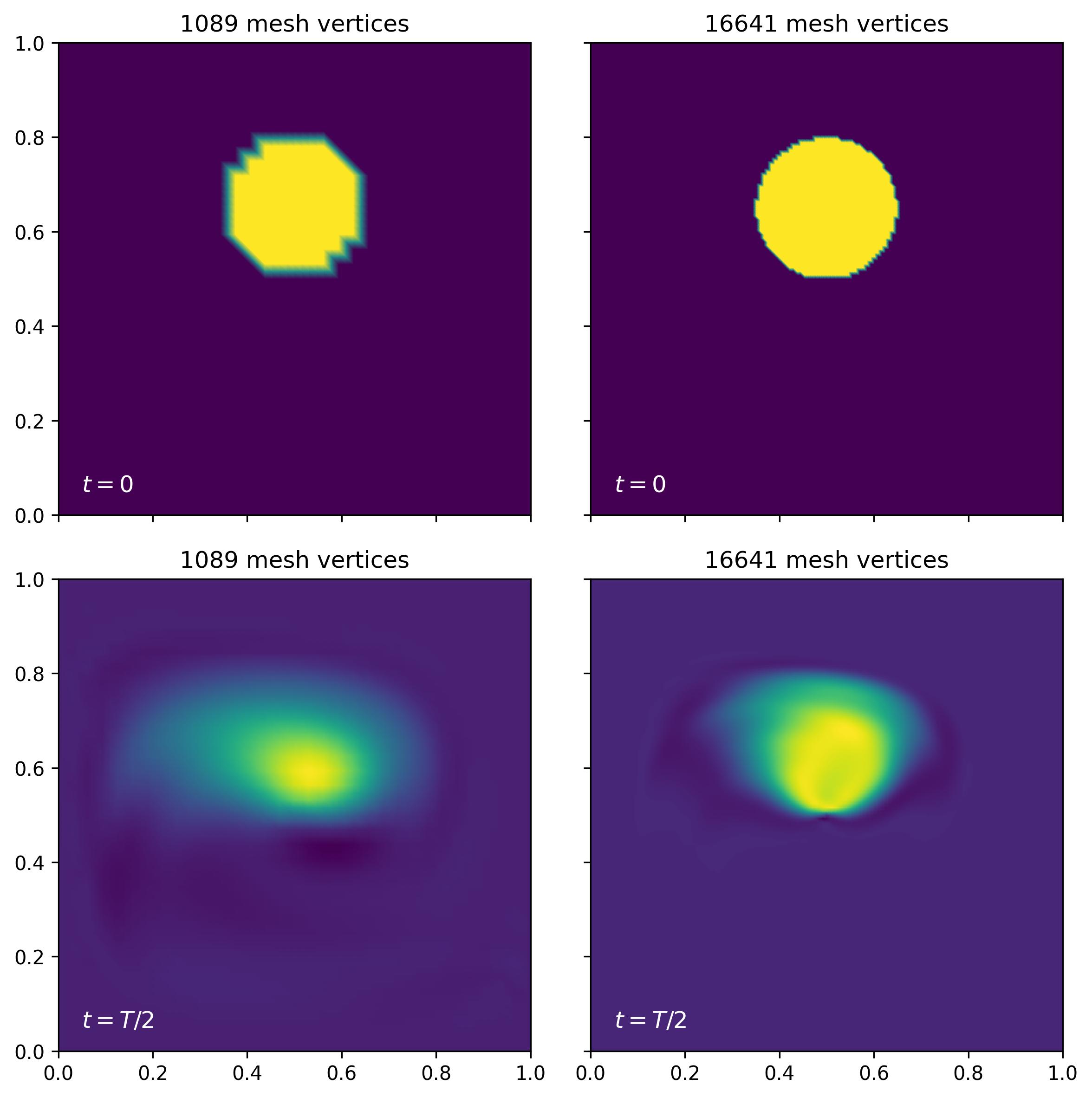
We can now compare computed final concentration fields on the two meshes to the initial condition.

import matplotlib.pyplot as plt
from firedrake.pyplot import *

fig, axes = plt.subplots(2, 2, figsize=(8, 8), sharex=True, sharey=True)
time_labels = [r"$t=0$", r"$t=T/2$"]
c_values = [[c0_coarse, c0_fine], [c_coarse_final, c_fine_final]]
meshes = [mesh_coarse, mesh_fine]
for i in range(2):
    for ax, c, mesh in zip(axes[i], c_values[i], meshes):
        im = tripcolor(c, axes=ax)
        ax.set_title(f"{mesh.num_vertices()} mesh vertices")
        ax.text(0.05, 0.05, time_labels[i], fontsize=12, color="white", ha="left")
        ax.set_xlim(0, 1)
        ax.set_ylim(0, 1)
        ax.set_aspect("equal")
fig.tight_layout()
fig.savefig("bubble_shear-uniform.jpg", dpi=300, bbox_inches="tight")

We observe that the concentration fields have not returned to their initial value at the end of the simulation, as we would have expected. This is particularly obvious in the coarse resolution simulation. This is due to the addition of the SUPG stabilisation to the weak form of the advection equation, which adds numerical diffusion. Numerical diffusion is necessary for numerical stability and for preventing oscillations, but it also makes the solution irreversible. The amount of difussion added is related to the grid Péclet number \(Pe = U\,h/2D\): the coarser the mesh is, the more diffusion is added.

In order to quantify the above observation, we will compute the relative \(L^2\) error between the initial condition and the final concentration field on the final mesh.

def compute_rel_error(c_init, c_final):
    init_l2_norm = norm(c_init, norm_type="L2")
    abs_l2_error = errornorm(c_init, c_final, norm_type="L2")
    return 100 * abs_l2_error / init_l2_norm


coarse_error = compute_rel_error(c0_coarse, c_coarse_final)
print(f"Relative L2 error on the coarse mesh: {coarse_error:.2f}%")
fine_error = compute_rel_error(c0_fine, c_fine_final)
print(f"Relative L2 error on the fine mesh: {fine_error:.2f}%.")

Relative L2 error on the coarse mesh: 56.52%
Relative L2 error on the fine mesh: 32.29%

Since accurate simulations require very fine resolution, which may be computationally too prohitibive, we will now demonstrate how to use mesh adaptation techniques to refine the mesh only in regions and at times where that is necessary. For the purposes of this demo, we are going to adapt the mesh 15 times throughout the simulation, at equal time intervals (i.e., every 0.2s of simulation time).

num_adaptations = 15
interval_length = simulation_end_time / num_adaptations

We will also define a function that will allow us to easily plot the adapted mesh, as well as the solution fields at the beginning and end of each subinterval.

def plot_mesh(mesh, c0, c1, i, method):
    fig, ax = plt.subplots(1, 3, sharey=True, figsize=(12, 4))
    triplot(mesh, axes=ax[0])
    tripcolor(c0, axes=ax[1])
    tripcolor(c1, axes=ax[2])
    ax[0].set_title(f"Mesh {i} ({mesh.num_vertices()} vertices)")
    ax[1].set_title(f"Solution at t={i*interval_length:.1f}s")
    ax[2].set_title(f"Solution at t={(i+1)*interval_length:.1f}s")
    for axes in ax:
        axes.set_xlim(0, 1)
        axes.set_ylim(0, 1)
        axes.set_aspect("equal")
    fig.savefig(f"bubble_shear-{method}_{i}.jpg", dpi=300, bbox_inches="tight")
    plt.close(fig)

As mentioned in the introduction, we shall demonstrate two different mesh adaptation strategies. Let us begin with the classical mesh adaptation algorithm, which adapts each mesh before solving the advection equation over the corresponding subinterval. Here we will use the RiemannianMetric class to define the metric, which we will compute based on the Hessian of the concentration field. Let us therefore define a function which takes the original mesh and the concentration field as arguments, and returns the adapted mesh. We will also define parameters for computing the metric.

from animate.adapt import adapt
from animate.metric import RiemannianMetric

metric_params = {
    "dm_plex_metric": {
        "target_complexity": 1500.0,
        "p": 2.0,  # normalisation order
        "h_min": 1e-04,  # minimum allowed edge length
        "h_max": 1.0,  # maximum allowed edge length
    }
}


def adapt_classical(mesh, c):
    P1_ten = TensorFunctionSpace(mesh, "CG", 1)
    metric = RiemannianMetric(P1_ten)
    metric.set_parameters(metric_params)
    metric.compute_hessian(c)
    metric.normalise()
    adapted_mesh = adapt(mesh, metric)
    return adapted_mesh

We can now run the simulation, but we adapt the mesh before each subinterval. We begin with a coarse uniform mesh and track the number of vertices of each adapted mesh.

mesh = UnitSquareMesh(32, 32)
mesh_numVertices = []
c = get_initial_condition(mesh)
for i in range(num_adaptations):
    t0 = i * interval_length  # subinterval start time
    t1 = (i + 1) * interval_length  # subinterval end time

    # Adapt the mesh based on the concentration field at t0
    mesh = adapt_classical(mesh, c)
    mesh_numVertices.append(mesh.num_vertices())

    # Make a copy of the initial condition for plotting purposes
    c0 = c.copy(deepcopy=True)

    # Solve the advection equation over the subinterval (t0, t1]
    c = run_simulation(mesh, t0, t1, c)

    # Plot the adapted mesh and the concentration field at t0 and t1
    plot_mesh(mesh, c0, c, i, "classical")

Now let us examine the final adapted mesh and final concentration field computed on it. We will also compute the relative \(L^2\) error.

# Redefine the initial condition on the final adapted mesh
c0 = get_initial_condition(mesh)
classical_c0 = Function(FunctionSpace(mesh, "CG", 1)).interpolate(c0)
classical_error = compute_rel_error(classical_c0, c)

print(
    f"Classical mesh adaptation.\n"
    f"   Avg. number of vertices: {np.average(mesh_numVertices):.1f}\n"
    f"   Relative L2 error: {classical_error:.2f}%"
)

Classical mesh adaptation.
   Avg. number of vertices: 2302.3
   Relative L2 error: 31.76%

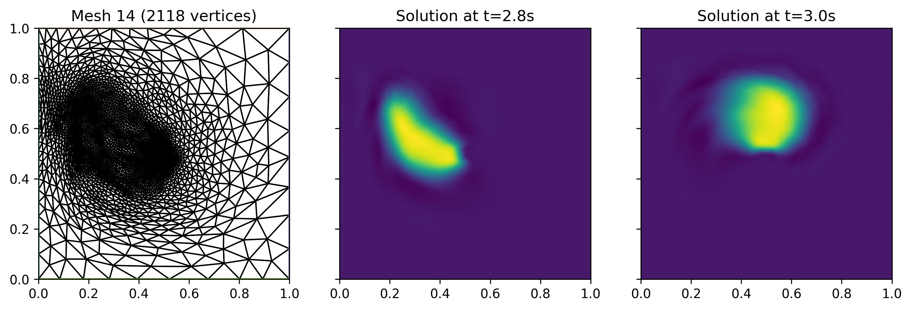
As we can see, the relative \(L^2\) error is lower than the one obtained with the uniform fine mesh, even though the average number of vertices is more than 8 times smaller. This demonstrates the effectiveness of mesh adaptation, which we can also observe in the figure above. We see that final mesh has clearly been refined around the bubble at the beginning of the final subinterval and coarsened elsewhere.

However, we also observe that the bubble has advected out of the fine resolution region by the end of the subinterval. This is a common occurence in time-dependent mesh adaptation, known as the lagging mesh problem, where the mesh is said to lag with respect to the solution. Ensuring that the bubble remains well-resolved throughout the simulation is not a trivial task, as it requires predicting where the bubble will be in the future. Earliest attempts at preventing the lagging mesh problem introduced a safety margin around the fine-resolution region. While potentially very effective, depending on the size of the margin, this approach is also likely to be inefficient as it may prescribe fine resolution in regions where it is not needed.

For advection-dominated problems, as is the case here, a metric advection algorithm has been proposed in []. The idea is to still compute the metric based on the solution at the current time, but then to advect the metric along the flow in order to predict where to prescribe fine resolution in the future. By combining the advected metrics in time, we obtain a final metric that is representative of the evolving solution throughout the subinterval. We achieve this in the following function, where we solve the before-seen advection equation for each component of the metric tensor.

def adapt_metric_advection(mesh, t_start, t_end, c):
    P1_ten = TensorFunctionSpace(mesh, "CG", 1)
    m = RiemannianMetric(P1_ten)  # metric at current timestep
    m_ = RiemannianMetric(P1_ten)  # metric at previous timestep
    metric_intersect = RiemannianMetric(P1_ten)

    # Compute the Hessian metric at t_start
    for mtrc in [m, m_, metric_intersect]:
        mtrc.set_parameters(metric_params)
    m_.compute_hessian(c)
    m_.enforce_spd(restrict_sizes=True, restrict_anisotropy=True)

    # Set the boundary condition for the metric tensor
    h_bc = Function(P1_ten)
    h_max = metric_params["dm_plex_metric"]["h_max"]
    h_bc.interpolate(Constant([[1.0 / h_max**2, 0.0], [0.0, 1.0 / h_max**2]]))

    V = VectorFunctionSpace(mesh, "CG", 1)
    u = Function(V)
    u_ = Function(V).interpolate(velocity_expression(mesh, t_start))

    R = FunctionSpace(mesh, "R", 0)
    dt = Function(R).assign(0.01)  # timestep size
    theta = Function(R).assign(0.5)  # Crank-Nicolson implicitness

    # SUPG stabilisation
    D = Function(R).assign(0.1)
    h = CellSize(mesh)
    U = sqrt(dot(u, u))
    tau = 0.5 * h / U
    tau = min_value(tau, U * h / (6 * D))

    # Apply SUPG stabilisation
    phi = TestFunction(P1_ten)
    phi += tau * dot(u, grad(phi))

    # Variational form of the advection equation for the metric tensor
    trial = TrialFunction(P1_ten)
    a = inner(trial, phi) * dx + dt * theta * inner(dot(u, grad(trial)), phi) * dx
    L = inner(m_, phi) * dx - dt * (1 - theta) * inner(dot(u_, grad(m_)), phi) * dx
    bcs = DirichletBC(P1_ten, h_bc, "on_boundary")
    lvp = LinearVariationalProblem(a, L, m, bcs=bcs)
    lvs = LinearVariationalSolver(lvp)

    # Integrate from t_start to t_end
    t = t_start + float(dt)
    while t < t_end + 0.5 * float(dt):
        u.interpolate(velocity_expression(mesh, t))

        lvs.solve()

        # Intersect metrics at every timestep
        m.enforce_spd(restrict_sizes=True, restrict_anisotropy=True)
        metric_intersect.intersect(m)

        # Update fields at the previous timestep
        m_.assign(m)
        u_.assign(u)
        t += float(dt)

    metric_intersect.normalise()
    amesh = adapt(mesh, metric_intersect)
    return amesh

We can now run the simulation over the entire time interval, but now we will adapt the mesh at the beginning of each subinterval using the metric advection algorithm.

mesh = UnitSquareMesh(32, 32)
mesh_numVertices = []
c = get_initial_condition(mesh)
for i in range(num_adaptations):
    t0 = i * interval_length  # subinterval start time
    t1 = (i + 1) * interval_length  # subinterval end time

    # Adapt the mesh based on the concentration field at t0
    mesh = adapt_metric_advection(mesh, t0, t1, c)
    mesh_numVertices.append(mesh.num_vertices())

    c0 = c.copy(deepcopy=True)

    # Solve the advection equation over the subinterval (t0, t1]
    c = run_simulation(mesh, t0, t1, c)

    plot_mesh(mesh, c0, c, i, "metric_advection")

c0 = get_initial_condition(mesh)
metric_adv_c0 = Function(FunctionSpace(mesh, "CG", 1)).interpolate(c0)
metric_adv_error = compute_rel_error(metric_adv_c0, c)

print(
    f"Metric advection mesh adaptation.\n"
    f"   Avg. number of vertices: {np.average(mesh_numVertices):.1f}\n"
    f"   Relative L2 error: {metric_adv_error:.2f}%"
)

Metric advection mesh adaptation.
   Avg. number of vertices: 2032.7
   Relative L2 error: 31.30%

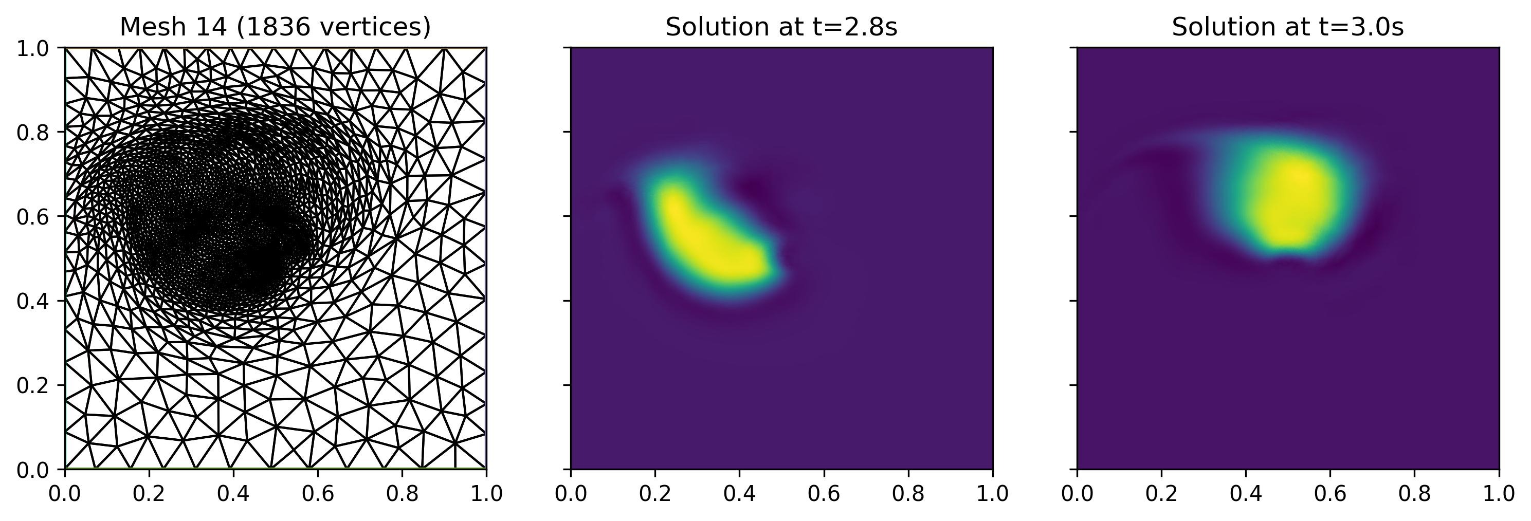
The relative \(L^2\) error of 31.30% is slightly lower than the one obtained with the classical mesh adaptation algorithm, but note that the average number of vertices is about 15% smaller. Looking into the final adapted mesh and concentration fields in the above figure, we now observe that the mesh is indeed refined in a much wider region - ensuring that the bubble remains well-resolved throughout the subinterval. However, this also means that the available resolution is more widely distributed, leading to a coarser local resolution compared to classical mesh adaptation.

Let us now consider the implications and limitations of each approach. Firstly, given a high enough adaptation frequency (i.e. number of adaptations/subintervals), the lagging mesh problem can be mitigated with the classical mesh adaptation algorithm. This may end up being more computationally efficient than the metric advection algorithm, which requires solving the advection equation once more at each timestep, as well as potentially expensive metric computations. However, while increasing the mesh adaptation frequency would alleviate the mesh lag, doing so may introduce large errors due to frequent solution transfers between meshes.

This is where the advantage of the metric advection algorithm lies: it predicts where to prescribe fine resolution in the future, and thus avoids the need for frequent solution transfers. We can assure ourselves of that by repeating the above simulations with num_adaptations = 5, which yields relative errors of 61.06% and 36.86% for the classical and metric advection algorithms, respectively. Conversely, increasing the adaptation frequency to num_adaptations = 50 yields again relative errors closer to one another. Note that the algorithms are identical if we adapt at every timestep. We summarise these results in the table below, noting also the average number of vertices, \(N_v\).

Number of adaptations	Classical (avg. \(N_v\))	Metric advection (avg. \(N_v\))
5	61.06% (2200.2)	36.86% (1922.2)
15	31.76% (2302.3)	31.30% (2032.7)
50	26.80% (2522.1)	27.99% (2166.3)

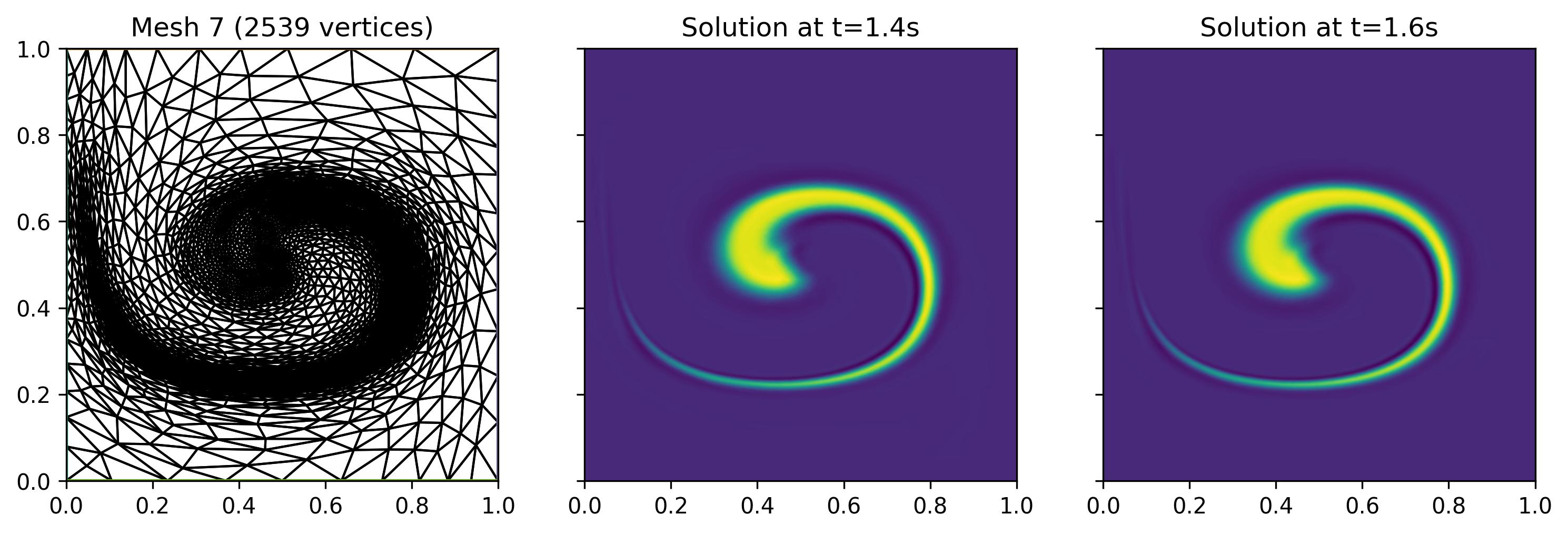
Furthermore, the problem considered in this example is relatively well-suited for classical mesh adaptation, as the bubble concentration field reverses and therefore often indeed remains in the finely-resolved region. We can observe that in the below figure, at the subinterval \((1.4 s, 1.6 s]\). This also means that the meshes adapted using classical and metric advection algorithms are qualitatively similar at this subinterval.

In conclusion, the choice of mesh adaptation algorithm depends on the specific problem at hand, as well as the computational resources available.

Exercise

Repeat above experiments and investigate each of the adapted meshes. At what subintervals do the two algorithms produce most similar and most different meshes? Experiment with different metric parameters, different adaptation frequencies, and even different velocity fields to further explore the capabilities and limitations of the algorithms presented above.

This demo can also be accessed as a Python script.