Error estimation for Burgers equation

So far, we have learnt how to set up MeshSeqs and solve forward and adjoint problems. In this demo, we use this functionality to perform goal-oriented error estimation.

The fundamental result in goal-oriented error estimation is the dual-weighted residual,

\[J(u)-J(u_h)\approx\rho(u_h,u^*),\]

where \(u\) is the solution of a PDE with weak residual \(\rho(\cdot,\cdot)\), \(u_h\) is a finite element solution and \(J\) is the quantity of interest (QoI). Here, the exact solution \(u^*\) of the associated adjoint problem replaces the test function in the second argument of the weak residual. In practice, we do not know what this is, of course. As such, it is common practice to evaluate the dual weighted residual by approximating the true adjoint solution in an enriched finite element space. That is, a superspace, obtained by adding more degrees of freedom to the base space. This could be done by solving global or local auxiliary PDEs, or by applying patch recovery type methods. Currently, only global enrichment is supported in Goalie.

from firedrake import *

from goalie_adjoint import *

set_log_level(DEBUG)

Redefine the field_names variable and the getter functions as in the first adjoint Burgers demo.

field_names = ["u"]


def get_function_spaces(mesh):
    return {"u": VectorFunctionSpace(mesh, "CG", 2)}


def get_form(mesh_seq):
    def form(index):
        u, u_ = mesh_seq.fields["u"]

        # Define constants
        R = FunctionSpace(mesh_seq[index], "R", 0)
        dt = Function(R).assign(mesh_seq.time_partition.timesteps[index])
        nu = Function(R).assign(0.0001)

        # Setup variational problem
        v = TestFunction(u.function_space())
        F = (
            inner((u - u_) / dt, v) * dx
            + inner(dot(u, nabla_grad(u)), v) * dx
            + nu * inner(grad(u), grad(v)) * dx
        )
        return {"u": F}

    return form


def get_solver(mesh_seq):
    def solver(index):
        u, u_ = mesh_seq.fields["u"]

        # Define form
        F = mesh_seq.form(index)["u"]

        # Time integrate from t_start to t_end
        P = mesh_seq.time_partition
        t_start, t_end = P.subintervals[index]
        dt = P.timesteps[index]
        t = t_start
        while t < t_end - 1.0e-05:
            solve(F == 0, u, ad_block_tag="u")
            yield

            u_.assign(u)
            t += dt

    return solver


def get_initial_condition(mesh_seq):
    fs = mesh_seq.function_spaces["u"][0]
    x, y = SpatialCoordinate(mesh_seq[0])
    return {"u": assemble(interpolate(as_vector([sin(pi * x), 0]), fs))}


def get_qoi(mesh_seq, i):
    def end_time_qoi():
        u = mesh_seq.fields["u"][0]
        return inner(u, u) * ds(2)

    return end_time_qoi

Next, create a sequence of meshes and a TimePartition.

n = 32
meshes = [UnitSquareMesh(n, n, diagonal="left"), UnitSquareMesh(n, n, diagonal="left")]
end_time = 0.5
dt = 1 / n
num_subintervals = len(meshes)
time_partition = TimePartition(
    end_time,
    num_subintervals,
    dt,
    field_names,
    num_timesteps_per_export=2,
)

A key difference between this demo and the previous ones is that we need to use a GoalOrientedMeshSeq to access the goal-oriented error estimation functionality. Note that GoalOrientedMeshSeq is a subclass of AdjointMeshSeq, which is a subclass of MeshSeq.

mesh_seq = GoalOrientedMeshSeq(
    time_partition,
    meshes,
    get_function_spaces=get_function_spaces,
    get_initial_condition=get_initial_condition,
    get_form=get_form,
    get_solver=get_solver,
    get_qoi=get_qoi,
    qoi_type="end_time",
)

Given the description of the PDE problem in the form of a GoalOrientedMeshSeq, Goalie is able to extract all of the relevant information to automatically compute error estimators. During the computation, we solve the forward and adjoint equations over the mesh sequence, as before. In addition, we solve the adjoint problem again in an enriched finite element space. Currently, Goalie supports uniform refinement of the meshes (\(h\)-refinement) or globally increasing the polynomial order (\(p\)-refinement). Choosing one (or both) of these as the "enrichment_method", we are able to compute error indicator fields as follows.

solutions, indicators = mesh_seq.indicate_errors(
    enrichment_kwargs={"enrichment_method": "h"}
)

An error indicator field \(i\) takes constant values on each mesh element, say \(i_K\) for element \(K\) of mesh \(\mathcal H\). It decomposes the global error estimator \(\epsilon\) into its local contributions.

\[\epsilon = \sum_{K\in\mathcal H}i_K \approx \rho(u_h,u^*).\]

For the purposes of this demo, we plot the solution at each exported timestep using the plotting driver function plot_indicator_snapshots().

fig, axes, tcs = plot_indicator_snapshots(indicators, time_partition, "u", levels=50)
fig.savefig("burgers-ee.jpg")

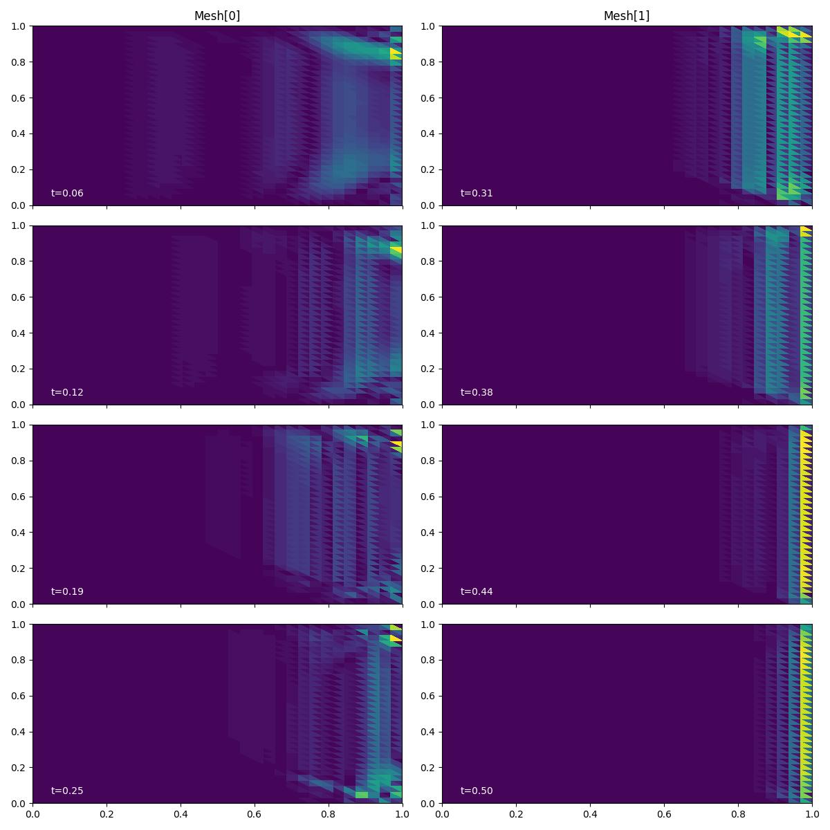
We observe that the contributions to the QoI error are estimated to be much higher in the right-hand part of the domain than the left. This makes sense, becase the QoI is evaluated along the right-hand boundary and we have already seen that the magnitude of the adjoint solution tends to be larger in that region, too.

Exercise

Try running the demo again, but with a "time_integrated" QoI, rather than an "end_time" one. How do the error indicator fields change in this case?

This demo can also be accessed as a Python script.