Mesh movement using Laplacian smoothing

In this demo, we demonstrate the Laplacian smoothing approach. This method relies on there being a user-specified boundary condition. With this, we can define a vector Laplace equation of the form

\[-\Delta_{\boldsymbol{\xi}}\mathbf{v} = \boldsymbol{0},\]

where \(\mathbf{v}\) is the so-called mesh velocity that we solve for. Note that the derivatives in the Laplace equation are in terms of the computational coordinates \(\boldsymbol{\xi}\), rather than the physical coordinates \(\mathbf{x}\).

With the mesh velocity, we update the physical coordinates according to

\[\mathbf{x} := \mathbf{x} + \mathbf{v} \Delta t,\]

where \(\Delta t\) is the timestep.

To motivate why we might want to take this sort of approach, consider momentarily the 1D case, where we have velocities \(\{v_i\}_{i=1}^n\) at each of a sequence of \(n\in\mathbb{N}\) points with uniform separation \(h\). If we want to smooth out the local variation in the velocities in the vicinity of \(v_i\), we might consider averaging out \((v_{i-1}-v_i)/h\) and \((v_{i+1}-v_i)/h\). Doing so gives

\[\frac1h(\frac{v_{i-1}-v_i}{h} + \frac{v_{i+1}-v_i}{h}) = 0,\]

i.e.,

\[\frac1{h^2}(-v_{i-1} + 2v_i - v_{i+1}) = 0,\]

the left-hand side of which you might recognise as a finite difference approximation of the second derivative, i.e., the Laplace operator.

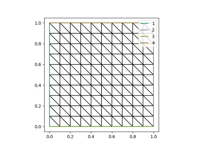
Let’s start with a uniform mesh of the unit square. It has four boundary segments, which are tagged with the integers 1, 2, 3, and 4. Note that segment 4 corresponds to the top boundary.

import matplotlib.pyplot as plt
from firedrake import *
from firedrake.pyplot import triplot

from movement import *

n = 10
mesh = UnitSquareMesh(n, n)
coord_data_init = mesh.coordinates.dat.data.copy()
fig, axes = plt.subplots()
triplot(mesh, axes=axes)
axes.set_aspect(1)
axes.legend()
plt.savefig("laplacian_smoothing-initial_mesh.jpg")

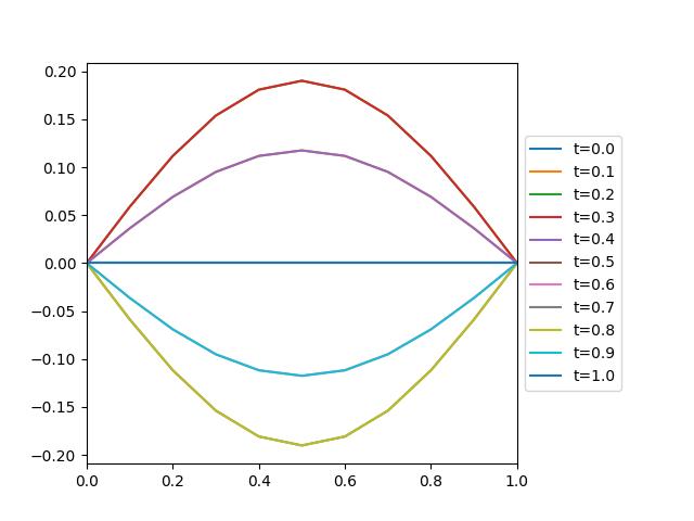
Suppose we wish to enforce a time-dependent velocity \(\mathbf{v}_f\) on the top boundary and see how the mesh responds. Consider the velocity

\[\mathbf{v}_f(x,y,t) = \left[0, A\:\sin\left(\frac{2\pi t}T\right)\:\sin(\pi x)\right]\]

acting only in the vertical direction, where \(A\) is the amplitude and \(T\) is the time period. The displacement follows a sinusoidal pattern along that boundary. The boundary movement is also sinusoidal in time, such that it ramps up and then reverses, with the analytical solution being that the final mesh coincides with the initial mesh.

import numpy as np

bv_period = 1.0
num_timesteps = 10
timestep = bv_period / num_timesteps
bv_amplitude = 0.2


def boundary_velocity(x, t):
    return bv_amplitude * np.sin(2 * pi * t / bv_period) * np.sin(pi * x)


X = np.linspace(0, 1, n + 1)
times = np.arange(0, bv_period + 0.5 * timestep, timestep)

fig, axes = plt.subplots()
for time in times:
    axes.plot(X, boundary_velocity(X, time), label=f"t={time:.1f}")
axes.set_xlim([0, 1])
axes.legend()
box = axes.get_position()
axes.set_position([box.x0, box.y0, box.width * 0.8, box.height])
axes.legend(loc="center left", bbox_to_anchor=(1, 0.5))
plt.savefig("laplacian_smoothing-boundary_velocity.jpg")

To enforce this boundary velocity, we need to create a LaplacianSmoother instance and define a function for updating the boundary conditions. Since we are going to enforce the velocity on the top boundary, we create a Function to represent the boundary condition values and pass this to a DirichletBC object. We then define a function which updates it as time progresses.

mover = LaplacianSmoother(mesh, timestep)
top = Function(mover.coord_space)
moving_boundary = DirichletBC(mover.coord_space, top, 4)


def update_boundary_velocity(t):
    coord_data = mesh.coordinates.dat.data
    bv_data = top.dat.data
    for i in moving_boundary.nodes:
        x, y = coord_data[i]
        bv_data[i][1] = boundary_velocity(x, t)

In addition to the moving boundary, we specify the remaining boundaries to be fixed.

fixed_boundaries = DirichletBC(mover.coord_space, 0, [1, 2, 3])
boundary_conditions = (fixed_boundaries, moving_boundary)

We are now able to apply the mesh movement method, passing the update_boundary_velocity function and boundary_conditions tuple to the move() method.

import matplotlib.patches as mpatches

fig, axes = plt.subplots(ncols=4, nrows=3, figsize=(12, 10))
for i, time in enumerate(times):
    idx = 0 if i == 0 else (i + 1)

    # Move the mesh and calculate the displacement
    mover.move(
        time,
        update_boundary_velocity=update_boundary_velocity,
        boundary_conditions=boundary_conditions,
    )
    displacement = np.linalg.norm(mover.displacement)
    print(f"time = {time:.1f} s, displacement = {displacement:.2f} m")

    # Plot the current mesh, adding a time label
    ax = axes[idx // 4, idx % 4]
    triplot(mover.mesh, axes=ax)
    ax.legend(handles=[mpatches.Patch(label=f"t={time:.1f}")], handlelength=0)
    ax.set_ylim([-0.05, 1.45])
axes[0, 1].axis(False)
plt.savefig("laplacian_smoothing-adapted_meshes.jpg")

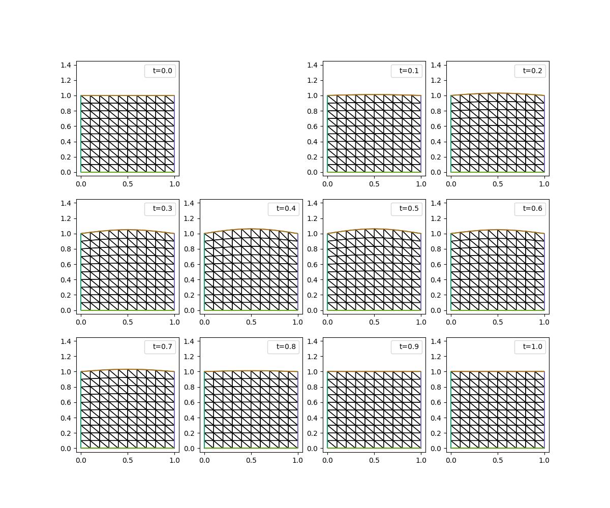
The mesh is deformed according to the vertical velocity on the top boundary, with the left, right, and bottom boundaries remaining fixed, returning it to be very close to its original state after one period. Let’s check this in the \(\ell_\infty\) norm.

coord_data = mover.mesh.coordinates.dat.data
linf_error = np.max(np.abs(coord_data - coord_data_init))
print(f"l_infinity error: {linf_error:.3f} m")
assert np.isclose(linf_error, 0.0)

l_infinity error: 0.000 m

This tutorial can be downloaded as a Python script.