Methods for interpolating fields between different meshes
In this demo, we perform a ‘ping pong test’, which amounts to interpolating a given source function repeatedly between the two meshes using a particular interpolation method. The purpose of this experiment is to assess the properties of different interpolation methods.
import matplotlib.pyplot as plt
from firedrake import *
from firedrake.pyplot import tricontourf, triplot

from animate import *
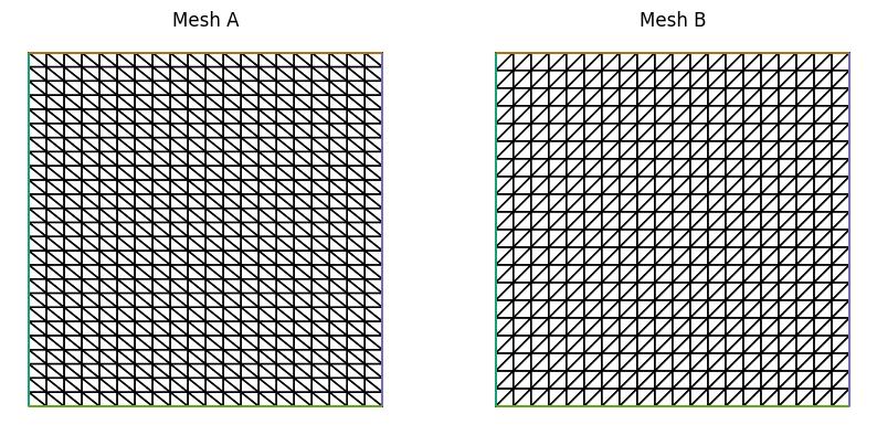
Consider two different meshes of the unit square: mesh A, which is laid out \(20\times25\) with diagonals from top left to bottom right and mesh B, which is laid out \(20\times20\) with diagonals from bottom left to top right. Note that mesh A has higher resolution in the vertical direction.
mesh_A = UnitSquareMesh(20, 25, diagonal="left", name="Mesh A")
mesh_B = UnitSquareMesh(20, 20, diagonal="right", name="Mesh B")

fig, axes = plt.subplots(ncols=2, figsize=(10, 5))
for i, mesh in enumerate((mesh_A, mesh_B)):
    triplot(mesh, axes=axes[i])
    axes[i].set_title(mesh.name)
    axes[i].axis(False)
    axes[i].set_aspect(1)
plt.savefig("ping_pong-meshes.jpg", bbox_inches="tight")
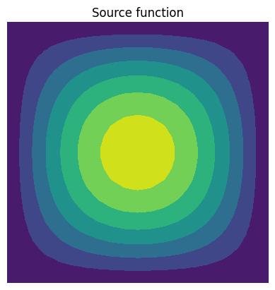
Define the source function
Let’s plot it as represented in \(\mathbb{P}1\) spaces on mesh A.
V_A = FunctionSpace(mesh_A, "CG", 1)
V_B = FunctionSpace(mesh_B, "CG", 1)
x, y = SpatialCoordinate(mesh_A)
source = Function(V_A, name="Source").interpolate(sin(pi * x) * sin(pi * y))

fig, axes = plt.subplots()
tricontourf(source, axes=axes)
axes.set_title("Source function")
axes.axis(False)
axes.set_aspect(1)
plt.savefig("ping_pong-source_function.jpg", bbox_inches="tight")
To start with, let’s consider the interpolate approach, which evaluates the input
field at the locations corresponding to degrees of freedom of the target function
space. We run the experiment for 50 iterations and track three quantities as the
iterations progress: the integral of the field, its global minimum, and its global
maximum.
niter = 50
initial_integral = assemble(source * dx)
initial_min = source.vector().gather().min()
initial_max = source.vector().gather().max()
quantities = {
    "integral": {"interpolate": [initial_integral]},
    "minimum": {"interpolate": [initial_min]},
    "maximum": {"interpolate": [initial_max]},
}
f_interp = Function(V_A).assign(source)
tmp = Function(V_B)
for _ in range(niter):
    interpolate(f_interp, tmp)
    interpolate(tmp, f_interp)
    quantities["integral"]["interpolate"].append(assemble(f_interp * dx))
    quantities["minimum"]["interpolate"].append(f_interp.vector().gather().min())
    quantities["maximum"]["interpolate"].append(f_interp.vector().gather().max())
f_interp.rename("Interpolate")

fig, axes = plt.subplots(ncols=3, figsize=(18, 5))
for i, (key, subdict) in enumerate(quantities.items()):
    axes[i].plot(subdict["interpolate"])
    axes[i].set_xlabel("Number of transfers back and forth")
    axes[i].set_ylabel(key.capitalize())
    axes[i].grid(True)
plt.savefig("ping_pong-quantities_interpolate.jpg", bbox_inches="tight")
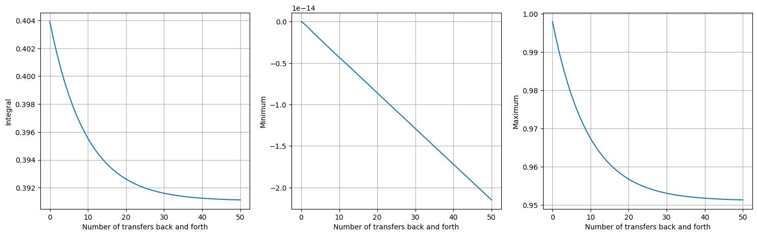
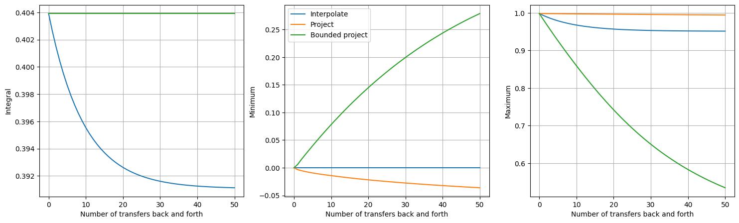
The first plot shows the integral of the field (i.e., the ‘mass’) as the interpolation iterations progress. Note that the mass drops steeply, before levelling out after around 50 iterations. Minimum values are perfectly maintained for this example, staying at zero for all iterations. Maximum values, however, decrease for several iterations before levelling out after around 30 iterations. The reason minima are attained but not maxima is that global minimum values are attained at the boundaries for this example, wheras the global maximum is attained at the centre of the domain.
In this example, we observe two general properties of the point interpolation method:
It is not conservative.
It does not introduce new extrema.
To elaborate on the second point, whilst the maximum value does decrease, new maxima are not introduced. Similarly, no new minima are introduced.
Next, we move on to the project approach, which uses the concept of a ‘supermesh’
to set up a conservative projection operator. The clue is in the name: we expect this
approach to conserve ‘mass’, i.e., the integral of the field. In fact, the approach
is designed to satisfy this property. Let \(f\in V_A\) denote the source field.
Then the projection operator, \(\Pi\), is chosen such that
This is achieved by solving the equation
for \(\boldsymbol{\pi}\) - the vector of data underlying \(\Pi(f)\) - where \(\mathbf{f}\) is the vector of data underlying \(f\), \(\underline{\mathbf{M}_B}\) is the mass matrix for the target space, \(V_B\), and \(\underline{\mathbf{M}_{BA}}\) is the mixed mass matrix mapping from the source space \(V_A\) to the target space.
quantities["integral"]["project"] = [initial_integral]
quantities["minimum"]["project"] = [initial_min]
quantities["maximum"]["project"] = [initial_max]
f_proj = Function(V_A).assign(source)
for _ in range(niter):
    project(f_proj, tmp)
    project(tmp, f_proj)
    quantities["integral"]["project"].append(assemble(f_proj * dx))
    quantities["minimum"]["project"].append(f_proj.vector().gather().min())
    quantities["maximum"]["project"].append(f_proj.vector().gather().max())
f_proj.rename("Project")

fig, axes = plt.subplots(ncols=3, figsize=(18, 5))
for i, (key, subdict) in enumerate(quantities.items()):
    axes[i].plot(subdict["interpolate"], label="Interpolate")
    axes[i].plot(subdict["project"], label="Project")
    axes[i].set_xlabel("Number of transfers back and forth")
    axes[i].set_ylabel(key.capitalize())
    axes[i].grid(True)
axes[1].legend()
plt.savefig("ping_pong-quantities_project.jpg", bbox_inches="tight")
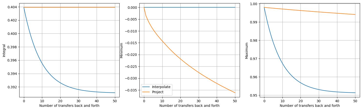
The first subfigure shows that mass is indeed conserved by the project approach,
unlike the interpolate approach. However, contrary to the interpolate approach
not introducing new extrema, the project approach can be seen to introduce new
minimum values. No new maximum values are introduced, although the maximum values do
decrease slightly. Extrema are not attained because the conservative projection
approach used here is known to be diffusive. The fact that new minima are introduced
is again due to those values being on the boundary.
To summarise, the project approach:
It is conservative.
It may introduce new extrema.
Note that neither of the approaches considered thus far provide an interpolation method that is both conservative and does not introduce new extrema. In the case of \(\mathbb P1\) fields specifically, it is possible to achieve this using ‘mass lumping’. Recall the linear system above. Lumping amounts to replacing the mass matrix \(\underline{\mathbf{M}_B}\) with a diagonal matrix, whose entries correspond to the sums over the corresponding mass matrix rows. (See [FPP+09] for details.)
The resulting bounded projection operator can be used in Animate by passing
bounded=True to the project function.
quantities["integral"]["bounded"] = [initial_integral]
quantities["minimum"]["bounded"] = [initial_min]
quantities["maximum"]["bounded"] = [initial_max]
f_bounded = Function(V_A).assign(source)
for _ in range(niter):
    project(f_bounded, tmp, bounded=True)
    project(tmp, f_bounded, bounded=True)
    quantities["integral"]["bounded"].append(assemble(f_bounded * dx))
    quantities["minimum"]["bounded"].append(f_bounded.vector().gather().min())
    quantities["maximum"]["bounded"].append(f_bounded.vector().gather().max())
f_bounded.rename("Bounded project")

fig, axes = plt.subplots(ncols=3, figsize=(18, 5))
for i, (key, subdict) in enumerate(quantities.items()):
    axes[i].plot(subdict["interpolate"], label="Interpolate")
    axes[i].plot(subdict["project"], label="Project")
    axes[i].plot(subdict["bounded"], label="Bounded project")
    axes[i].set_xlabel("Number of transfers back and forth")
    axes[i].set_ylabel(key.capitalize())
    axes[i].grid(True)
axes[1].legend()
plt.savefig("ping_pong-quantities_bounded.jpg", bbox_inches="tight")
To check that the interpolants still resemble the source function after 50 iterations, we plot the final fields alongside it.
fig, axes = plt.subplots(ncols=2, nrows=2, figsize=(10, 10))
levels = [-0.05, 0.0, 0.2, 0.4, 0.6, 0.8, 1.0, 1.05]
labels = ["<0.0", "0.0", "0.2", "0.4", "0.6", "0.8", "1.0", ">1.0"]
for ax, f in zip(axes.flatten(), (source, f_interp, f_proj, f_bounded)):
    ax.set_title(f.name())
    im = tricontourf(f, axes=ax, levels=levels)
    ax.axis(False)
    ax.set_aspect(1)
cbar = fig.colorbar(im, ax=axes, orientation="horizontal", fraction=0.046, pad=0.04)
cbar.set_ticks(levels)
cbar.set_ticklabels(labels)
plt.savefig("ping_pong-final.jpg", bbox_inches="tight")
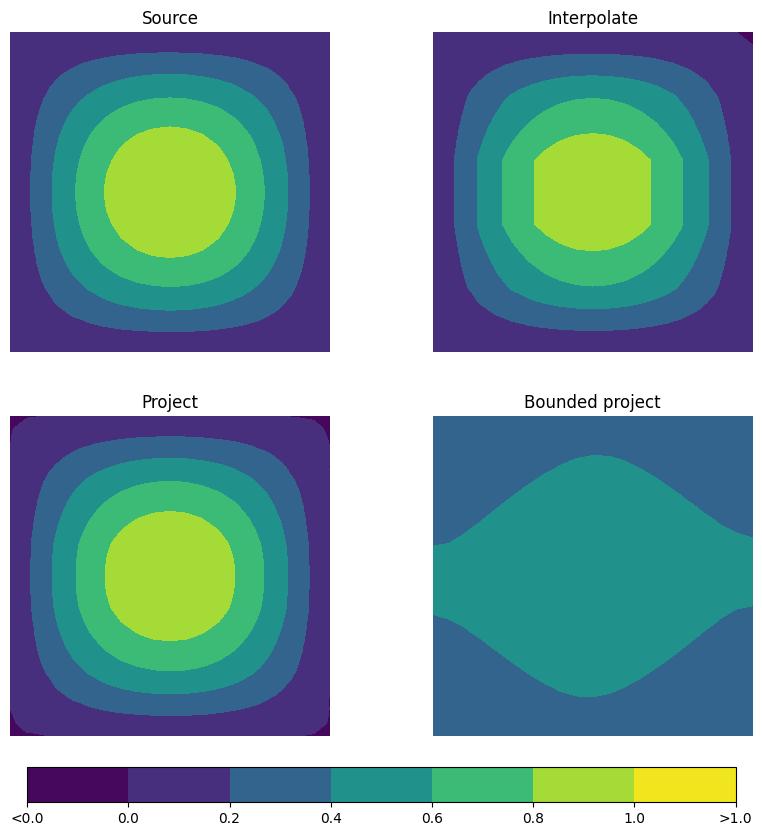
Whilst the first two approaches clearly resemble the input field, the bounded version gives a much poorer representation. This is because it introduces even more numerical diffusion than the standard conservative projection approach. As such, we find that, whilst the bounded conservative projection allows for an interpolation operator with attractive properties, we shouldn’t expect it to give smaller errors. To demonstrate this, we print the \(L^2\) errors for each method.
print(f"Interpolate:     {errornorm(source, f_interp):.4e}")
print(f"Project:         {errornorm(source, f_proj):.4e}")
print(f"Bounded project: {errornorm(source, f_bounded):.4e}")
Interpolate:     1.7144e-02
Project:         2.5693e-03
Bounded project: 2.3513e-01
This demo can also be accessed as a Python script.
References
Patrick E Farrell, Matthew D Piggott, Christopher C Pain, Gerard J Gorman, and Cian R Wilson. Conservative interpolation between unstructured meshes via supermesh construction. Computer methods in applied mechanics and engineering, 198(33-36):2632–2642, 2009.