Defining a simple metric field and adapting the mesh to it

Animate provides the RiemannianMetric class which is simply a firedrake.Function on a firedrake.TensorFunctionSpace with additional functionality. For metric-based mesh adaptivity the metric is usually assumed to be vertex-based, so we need to define the metric in a Continuous Galerkin (CG) P1 tensor function space

from firedrake import *
from firedrake.pyplot import triplot

from animate import *

mesh = UnitSquareMesh(10, 10)
P1_ten = TensorFunctionSpace(mesh, "CG", 1)
metric = RiemannianMetric(P1_ten)

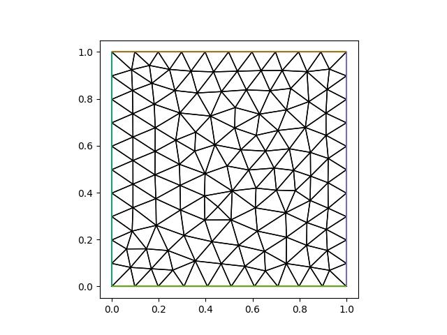
We start by choosing a uniform, and isotropic metric, which is to say that the metric tensor is just a constant diagonal matrix that is a scalar multiple of the identity matrix:

alpha = 100
metric.interpolate(as_matrix([[alpha, 0], [0, alpha]]))

In metric based adaptivity the metric is used to measure the length of edges: for any edge \(\mathbf e={\mathbf v_2}-{\mathbf v_1}\) written as a vector between vertices \(\mathbf v_1\) and \(\mathbf v_2\), its length in metric space is given by: .. math:

\ell_{\mathcal M}(\vec{\mathbf{e}})
:=\sqrt{\mathbf{e}^T{\mathcal M}\mathbf{e}}

which in this case evaluates to a simple scalar multiple of its Euclidean length: .. math:

\ell_{\mathcal M}(\vec{\mathbf{e}})
:=\sqrt{\mathbf{e}^T \begin{pmatrix} \alpha & 0 \\ 0 & \alpha \end{pmatrix} \mathbf{e}}
 =\sqrt{\alpha}~\sqrt{\mathbf{e}^T\mathbf{e}}.

The metric is used by the mesh adaptivity library to determine the optimal length of edges, where an edge is considered optimal if its length in metric space is 1. For our isotropic metric this means that an edge of (Euclidean) length \(h=\sqrt{\mathbf{e}^T\mathbf{e}}\) is considered optimal if \(\sqrt{\alpha} h=1\), or \(h=1/\sqrt{\alpha}\). Thus using \(\alpha=100\) we expect a mesh with edges of length \(h=0.1\)

new_mesh = adapt(mesh, metric)
import matplotlib.pyplot as plt

fig, axes = plt.subplots()
triplot(new_mesh, axes=axes)
axes.set_aspect("equal")
fig.show()
fig.savefig("simple_metric-mesh1.jpg")

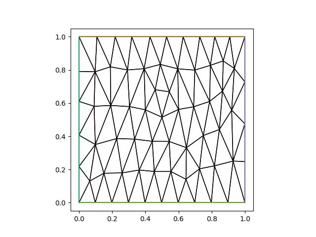
To create a anisotropic mesh with edge lengths \(h_x=0.1\) in the x-direction, and \(h_y=0.25\) we simply create a diagonal Riemannian metric with, respectively, the values \(1/0.1^2\) and \(1/0.25^2\) along the diagonal:

hx = 0.1
hy = 0.25
metric.interpolate(as_matrix([[1 / hx**2, 0], [0, 1 / hy**2]]))
new_mesh = adapt(mesh, metric)
fig, axes = plt.subplots()
triplot(new_mesh, axes=axes)
axes.set_aspect("equal")
fig.show()
fig.savefig("simple_metric-mesh2.jpg")

An example of a non-uniform mesh, in which we ask for higher resolution inside a circle of radius \(r\) is given below:

x, y = SpatialCoordinate(mesh)
r = 0.4
h1 = 0.02
h2 = 0.05
high = as_matrix([[1 / h1**2, 0], [0, 1 / h1**2]])
low = as_matrix([[1 / h2**2, 0], [0, 1 / h2**2]])
metric.interpolate(conditional(sqrt((x - 0.5) ** 2 + (y - 0.5) ** 2) < r, high, low))
new_mesh = adapt(mesh, metric)
fig, axes = plt.subplots(figsize=(16, 8), ncols=2)
triplot(mesh, axes=axes[0])
axes[0].set_aspect("equal")
axes[0].set_title("Input mesh: 10 x 10")
triplot(new_mesh, axes=axes[1])
axes[1].set_aspect("equal")
axes[1].set_title("Adapted mesh")
fig.show()
fig.savefig("simple_metric-mesh3.jpg")

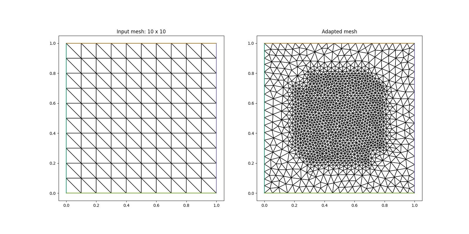
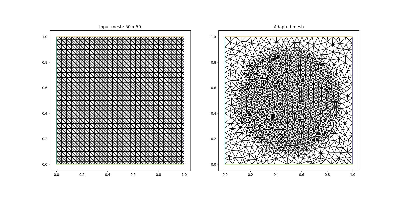
As we can observe in the figure on the right, the circular region of high resolution is not very accurately approximated. This is a consequence of the low resolution of the initial mesh (left figure) on which we have defined our metric. For a more accurate result we therefore increase the resolution of this initial mesh

mesh = UnitSquareMesh(50, 50)
P1_ten = TensorFunctionSpace(mesh, "CG", 1)
metric = RiemannianMetric(P1_ten)
x, y = SpatialCoordinate(mesh)
r = 0.4
h1 = 0.02
h2 = 0.05
high = as_matrix([[1 / h1**2, 0], [0, 1 / h1**2]])
low = as_matrix([[1 / h2**2, 0], [0, 1 / h2**2]])
metric.interpolate(conditional(sqrt((x - 0.5) ** 2 + (y - 0.5) ** 2) < r, high, low))
new_mesh = adapt(mesh, metric)
fig, axes = plt.subplots(figsize=(16, 8), ncols=2)
triplot(mesh, axes=axes[0])
axes[0].set_aspect("equal")
axes[0].set_title("Input mesh: 50 x 50")
triplot(new_mesh, axes=axes[1])
axes[1].set_aspect("equal")
axes[1].set_title("Adapted mesh")
fig.show()
fig.savefig("simple_metric-mesh4.jpg")

This demo can also be accessed as a Python script.