Solid body rotation

So far, we have only solved Burgers equation, which can be thought of as a nonlinear advection-diffusion equation. Let us now consider a simple linear advection equation,

\[\frac{\partial c}{\partial t} + \mathbf{u}\cdot\nabla c = 0,\]

which is solved for a tracer concentration \(c\). The velocity field \(\mathbf{u}\) drives the transport. Furthermore, we strongly impose zero Dirichlet boundary conditions:

\[c|_{\partial\Omega}=0,\]

where \(\Omega\) is the spatial domain of interest.

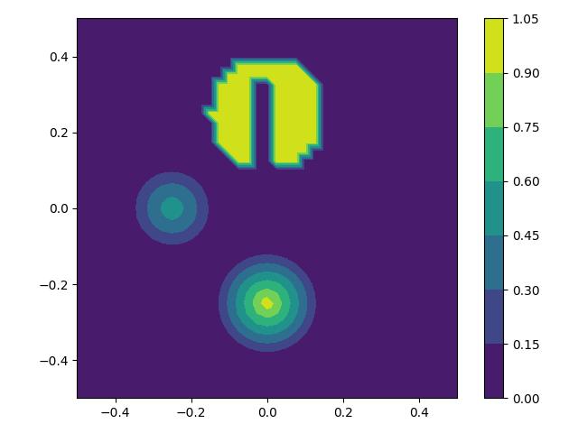
Consider the Firedrake DG advection demo. In this demo, a tracer is advected in a rotational velocity field such that its final concentration should be identical to its initial solution. If the tracer concentration is interpreted as a third spatial dimension, the initial condition is comprised of a Gaussian bell, a cone and a cylinder with a cuboid slot removed from it. The cone is more difficult to advect than the bell because of its discontinuous gradient at its peak and the slotted cylinder is yet more difficult to advect because of its curve of discontinuities. The test case was introduced in [LeV96].

As usual, we import from Firedrake and Goalie, with adjoint mode activated.

from firedrake import *

from goalie_adjoint import *

For simplicity, we use a \(\mathbb P1\) space for the concentration field. The domain of interest is again the unit square, in this case shifted to have its centre at the origin.

field_names = ["c"]


def get_function_spaces(mesh):
    return {"c": FunctionSpace(mesh, "CG", 1)}


mesh = UnitSquareMesh(40, 40)
coords = mesh.coordinates.copy(deepcopy=True)
coords.interpolate(coords - as_vector([0.5, 0.5]))
mesh = Mesh(coords)

Next, let’s define the initial condition, to get a better idea of the problem at hand.

def bell_initial_condition(x, y):
    bell_r0, bell_x0, bell_y0 = 0.15, -0.25, 0.0
    r = sqrt(pow(x - bell_x0, 2) + pow(y - bell_y0, 2))
    return 0.25 * (1 + cos(pi * min_value(r / bell_r0, 1.0)))


def cone_initial_condition(x, y):
    cone_r0, cone_x0, cone_y0 = 0.15, 0.0, -0.25
    return 1.0 - min_value(
        sqrt(pow(x - cone_x0, 2) + pow(y - cone_y0, 2)) / cone_r0, 1.0
    )


def slot_cyl_initial_condition(x, y):
    cyl_r0, cyl_x0, cyl_y0 = 0.15, 0.0, 0.25
    slot_left, slot_right, slot_top = -0.025, 0.025, 0.35
    return conditional(
        sqrt(pow(x - cyl_x0, 2) + pow(y - cyl_y0, 2)) < cyl_r0,
        conditional(And(And(x > slot_left, x < slot_right), y < slot_top), 0.0, 1.0),
        0.0,
    )


def get_initial_condition(mesh_seq):
    fs = mesh_seq.function_spaces["c"][0]
    x, y = SpatialCoordinate(mesh_seq[0])
    bell = bell_initial_condition(x, y)
    cone = cone_initial_condition(x, y)
    slot_cyl = slot_cyl_initial_condition(x, y)
    return {"c": assemble(interpolate(bell + cone + slot_cyl, fs))}

Now let’s set up the time interval of interest.

end_time = 2 * pi
dt = pi / 300
time_partition = TimeInterval(
    end_time,
    dt,
    field_names,
    num_timesteps_per_export=25,
)

For the purposes of plotting, we set up a MeshSeq with only the get_function_spaces() and get_initial_condition() methods implemented.

import matplotlib.pyplot as plt
from firedrake.pyplot import tricontourf

mesh_seq = MeshSeq(
    time_partition,
    mesh,
    get_function_spaces=get_function_spaces,
    get_initial_condition=get_initial_condition,
)

c_init = mesh_seq.get_initial_condition()["c"]

fig, axes = plt.subplots()
tc = tricontourf(c_init, axes=axes)
fig.colorbar(tc)
axes.set_aspect("equal")
plt.tight_layout()
plt.savefig("solid_body_rotation-init.jpg")

Now let’s set up the solver. First, we need to write the get_form() method. There is no integration by parts and we apply Crank-Nicolson timestepping with implicitness one half. Since we have a linear PDE, we write the variational problem in terms of a left-hand side and right-hand side and output both of them.

def get_form(mesh_seq):
    def form(index):
        c, c_ = mesh_seq.fields["c"]
        V = mesh_seq.function_spaces["c"][index]
        mesh = mesh_seq[index]

        # Define velocity field
        x, y = SpatialCoordinate(mesh)
        u = as_vector([-y, x])

        # Define constants
        R = FunctionSpace(mesh_seq[index], "R", 0)
        dt = Function(R).assign(mesh_seq.time_partition.timesteps[index])
        theta = Function(R).assign(0.5)

        psi = TrialFunction(V)
        phi = TestFunction(V)
        a = psi * phi * dx + dt * theta * dot(u, grad(psi)) * phi * dx
        L = c_ * phi * dx - dt * (1 - theta) * dot(u, grad(c_)) * phi * dx
        return {"c": (a, L)}

    return form

The get_form() function is then used by get_solver().

def get_solver(mesh_seq):
    def solver(index):
        function_space = mesh_seq.function_spaces["c"][index]
        c, c_ = mesh_seq.fields["c"]

        # Setup variational problem
        a, L = mesh_seq.form(index)["c"]

        # Zero Dirichlet condition on the boundary
        bcs = DirichletBC(function_space, 0, "on_boundary")

        # Setup the solver object
        lvp = LinearVariationalProblem(a, L, c, bcs=bcs)
        lvs = LinearVariationalSolver(lvp, ad_block_tag="c")

        # Time integrate from t_start to t_end
        tp = mesh_seq.time_partition
        t_start, t_end = tp.subintervals[index]
        dt = tp.timesteps[index]
        t = t_start
        while t < t_end - 0.5 * dt:
            lvs.solve()
            yield

            c_.assign(c)
            t += dt

    return solver

Note that we use a LinearVariationalSolver object and its solve() method, rather than calling the solve() function at every timestep because this avoids reassembling the various components and is therefore more efficient.

Finally, we need to set up the QoI, taken here to be the integral over a disc where the slotted cylinder is expected to be positioned at the end time.

def get_qoi(mesh_seq, index):
    def qoi():
        c = mesh_seq.fields["c"][0]
        x, y = SpatialCoordinate(mesh_seq[index])
        x0, y0, r0 = 0.0, 0.25, 0.15
        ball = conditional((x - x0) ** 2 + (y - y0) ** 2 < r0**2, 1.0, 0.0)
        return ball * c * dx

    return qoi

We are now ready to create an AdjointMeshSeq.

mesh_seq = AdjointMeshSeq(
    time_partition,
    mesh,
    get_function_spaces=get_function_spaces,
    get_initial_condition=get_initial_condition,
    get_form=get_form,
    get_solver=get_solver,
    get_qoi=get_qoi,
    qoi_type="end_time",
)
solutions = mesh_seq.solve_adjoint()

So far, we have visualised outputs using Matplotlib. In many cases, it is better to use Paraview. To save all adjoint solution components in Paraview format, use the following.

for field, sols in solutions.items():
    fwd_outfile = VTKFile(f"solid_body_rotation/{field}_forward.pvd")
    adj_outfile = VTKFile(f"solid_body_rotation/{field}_adjoint.pvd")
    for i in range(len(mesh_seq)):
        for sol in sols["forward"][i]:
            fwd_outfile.write(sol)
        for sol in sols["adjoint"][i]:
            adj_outfile.write(sol)

In the next demo, we increase the complexity by considering two concentration fields in an advection-diffusion-reaction problem.

This tutorial can be dowloaded as a Python script.

References

[LeV96]

Randall J. LeVeque. High-Resolution Conservative Algorithms for Advection in Incompressible Flow. SIAM Journal on Numerical Analysis, 33(2):627–665, 1996. doi:10.1137/0733033.