Mantle convection modelling
In all demos that we have considered so far, the equations that we have solved all involve a time derivative. Those are clearly time-dependent equations. However, time-dependent equations need not involve a time derivative. For example, they might include fields that vary with time. Examples of where this might happen are in continuous pressure projection approaches, ice sheet and glaciological modelling, and mantle convection modelling. In this demo, we illustrate how Goalie can be used to solve such problems.
We consider the problem of a mantle convection in a 2D unit square domain. The governing equations and Firedrake implementation are based on the 2D Cartesian incompressible isoviscous case from [Davies et al., 2022]. We refer the reader to the paper for a detailed description of the problem and implementation. Here we present the governing equations involving a Stokes system and an energy equation, which we solve for the velocity \(\mathbf{u}\), pressure \(p\), and temperature \(T\):
where \(\mu\), \(\kappa\), and \(\mathrm{Ra}\) are constant viscosity, thermal diffusivity, and Rayleigh number, respectively, and \(\mathbf{k}\) is the unit vector in the direction opposite to gravity. Note that while the Stokes equations do not involve a time derivative, they are still time-dependent as they depend on the temperature field \(T\), which is time-dependent.
As always, we begin by importing Firedrake and Goalie, and defining constants.
from firedrake import *

from goalie import *

Ra, mu, kappa = Constant(1e4), Constant(1.0), Constant(1.0)
k = Constant((0, 1))
The problem is solved simultaneously for the velocity \(\mathbf{u}\) and pressure \(p\) using a mixed formulation, which was introduced in a previous demo on advection-diffusion reaction.
To account for the lack of time derivative in the Stokes equations, we set the
unsteady keyword argument of the initialiser for the Field class to
False rather than the default True value to specify that the "up"
field is steady (i.e. without a time derivative). The T field is unsteady
(i.e. involves a time derivative) so we can use unsteady=True. Again, given the
mixed finite element space used for velocity, it is more convenient to define the
finite elements and pass these directly to the Field constructor.
p2v_element = VectorElement(FiniteElement("Lagrange", triangle, 2), dim=2)
p1_element = FiniteElement("Lagrange", triangle, 1)
fields = [
    Field("up", finite_element=MixedElement([p2v_element, p1_element]), unsteady=False),
    Field("T", finite_element=p1_element, unsteady=True),
]
We must set initial conditions to solve the problem. Note that we define the initial
condition for the mixed field "up" despite the equations not involving a time
derivative. In this case, the prescribed initial condition should be understood as the
initial guess for the solver.
def get_initial_condition(mesh_seq):
    x, y = SpatialCoordinate(mesh_seq[0])
    T_init = Function(mesh_seq.function_spaces["T"][0])
    T_init.interpolate(1.0 - y + 0.05 * cos(pi * x) * sin(pi * y))
    up_init = Function(mesh_seq.function_spaces["up"][0])  # Zero by default
    return {"up": up_init, "T": T_init}
In the solver, weak forms for the Stokes and energy equations are defined as follows.
Note that the mixed field "up" does not have a lagged term.
def get_solver(mesh_seq):
    def solver(index):
        Z = mesh_seq.function_spaces["up"][index]
        Q = mesh_seq.function_spaces["T"][index]

        up = mesh_seq.field_functions["up"]
        u, p = split(up)
        T, T_ = mesh_seq.field_functions["T"]

        # Crank-Nicolson time discretisation for temperature
        Ttheta = 0.5 * (T + T_)

        # Variational problem for the Stokes equations
        v, w = TestFunctions(mesh_seq.function_spaces["up"][index])
        stress = 2 * mu * sym(grad(u))
        F_up = (
            inner(grad(v), stress) * dx
            - div(v) * p * dx
            - (dot(v, k) * Ra * Ttheta) * dx
        )
        F_up += -w * div(u) * dx  # Continuity equation

        # Variational problem for the energy equation
        q = TestFunction(mesh_seq.function_spaces["T"][index])
        F_T = (
            q * (T - T_) / dt * dx
            + q * dot(u, grad(Ttheta)) * dx
            + dot(grad(q), kappa * grad(Ttheta)) * dx
        )

        # Boundary IDs
        left, right, bottom, top = 1, 2, 3, 4
        # Boundary conditions for velocity
        bcux = DirichletBC(Z.sub(0).sub(0), 0, sub_domain=(left, right))
        bcuy = DirichletBC(Z.sub(0).sub(1), 0, sub_domain=(bottom, top))
        bcs_up = [bcux, bcuy]
        # Boundary conditions for temperature
        bctb = DirichletBC(Q, 1.0, sub_domain=bottom)
        bctt = DirichletBC(Q, 0.0, sub_domain=top)
        bcs_T = [bctb, bctt]

        # Solver parameters dictionary
        solver_parameters = {
            "mat_type": "aij",
            "snes_type": "ksponly",
            "ksp_type": "preonly",
            "pc_type": "lu",
            "pc_factor_mat_solver_type": "mumps",
        }

        nlvp_up = NonlinearVariationalProblem(F_up, up, bcs=bcs_up)
        nlvs_up = NonlinearVariationalSolver(
            nlvp_up,
            solver_parameters=solver_parameters,
            ad_block_tag="up",
        )
        nlvp_T = NonlinearVariationalProblem(F_T, T, bcs=bcs_T)
        nlvs_T = NonlinearVariationalSolver(
            nlvp_T,
            solver_parameters=solver_parameters,
            ad_block_tag="T",
        )

        # Time integrate over the subinterval
        num_timesteps = mesh_seq.time_partition.num_timesteps_per_subinterval[index]
        for _ in range(num_timesteps):
            nlvs_up.solve()
            nlvs_T.solve()
            yield
            T_.assign(T)

    return solver
We can now create a MeshSeq object and solve the forward problem. For demonstration purposes, we only consider two subintervals and a low number of timesteps.
num_subintervals = 2
meshes = [UnitSquareMesh(32, 32) for _ in range(num_subintervals)]

dt = 1e-3
num_timesteps = 40
end_time = dt * num_timesteps
dt_per_export = [10 for _ in range(num_subintervals)]

time_partition = TimePartition(
    end_time,
    num_subintervals,
    dt,
    fields,
    num_timesteps_per_export=dt_per_export,
)

mesh_seq = MeshSeq(
    time_partition,
    meshes,
    get_initial_condition=get_initial_condition,
    get_solver=get_solver,
    transfer_method="interpolate",
)

solutions = mesh_seq.solve_forward()
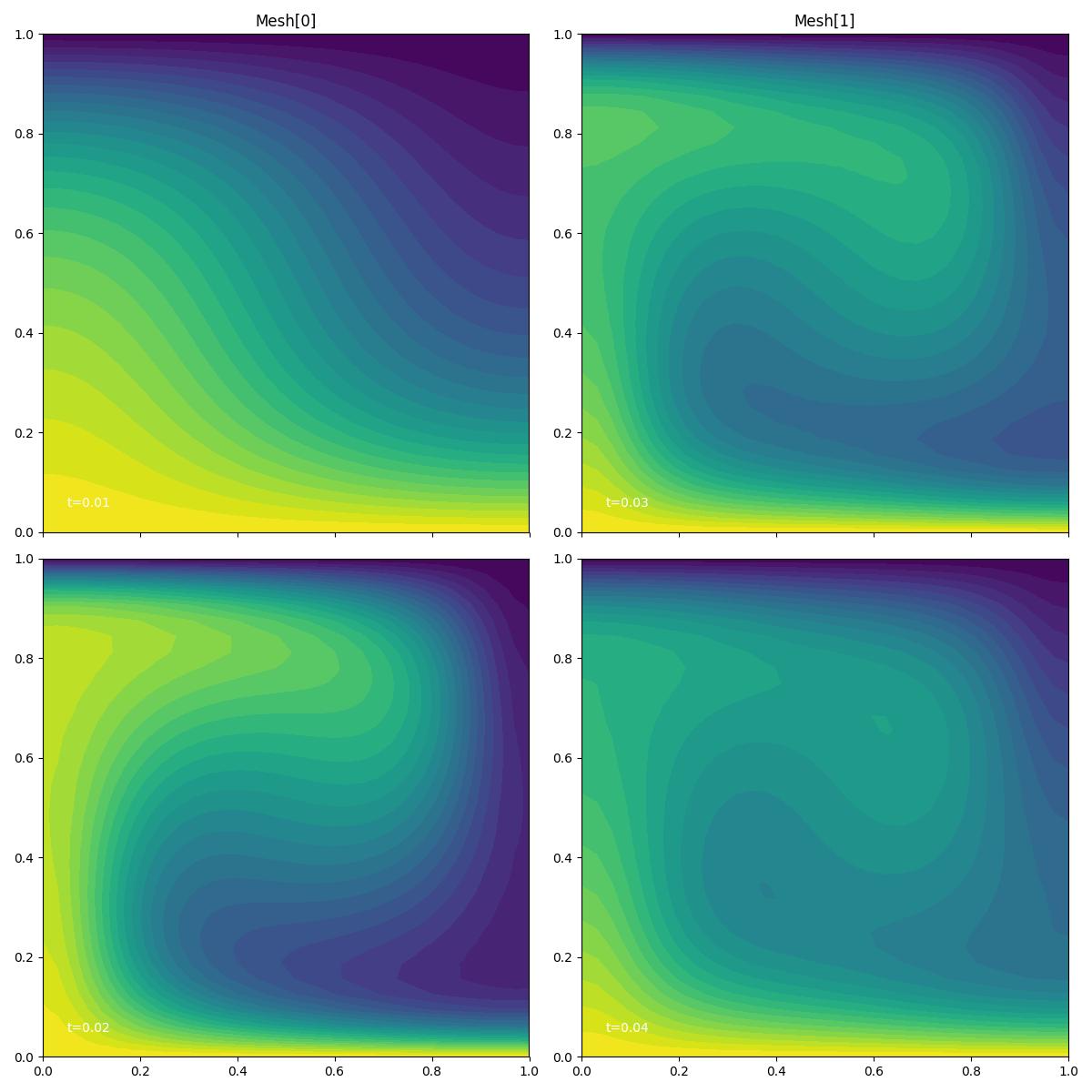
We can plot the temperature fields for exported timesteps using the in-built
plotting function plot_snapshots.
fig, axes, tcs = plot_snapshots(solutions, time_partition, "T", "forward", levels=25)
fig.savefig("mantle_convection.jpg")

This demo can also be accessed as a Python script.