Burgers equation with Hessian-based mesh adaptation
Yet again, we revisit the Burgers equation example. This time, we apply Hessian-based
mesh adaptation. The interesting thing about this demo is that, unlike the
previous demo and its predecessor,
we consider the time-dependent case. Moreover, we consider a MeshSeq with
multiple subintervals and hence multiple meshes to adapt.
As before, we copy over what is now effectively boiler plate to set up our problem.
import matplotlib.pyplot as plt
from animate.adapt import adapt
from animate.metric import RiemannianMetric
from firedrake import *

from goalie import *

field_names = ["u"]


def get_function_spaces(mesh):
    return {"u": VectorFunctionSpace(mesh, "CG", 2)}


def get_form(mesh_seq):
    def form(index):
        u, u_ = mesh_seq.fields["u"]

        # Define constants
        R = FunctionSpace(mesh_seq[index], "R", 0)
        dt = Function(R).assign(mesh_seq.time_partition.timesteps[index])
        nu = Function(R).assign(0.0001)

        # Setup variational problem
        v = TestFunction(u.function_space())
        F = (
            inner((u - u_) / dt, v) * dx
            + inner(dot(u, nabla_grad(u)), v) * dx
            + nu * inner(grad(u), grad(v)) * dx
        )
        return {"u": F}

    return form


def get_solver(mesh_seq):
    def solver(index):
        u, u_ = mesh_seq.fields["u"]

        # Define form
        F = mesh_seq.form(index)["u"]

        # Time integrate from t_start to t_end
        tp = mesh_seq.time_partition
        t_start, t_end = tp.subintervals[index]
        dt = tp.timesteps[index]
        t = t_start
        while t < t_end - 1.0e-05:
            solve(F == 0, u, ad_block_tag="u")
            yield

            u_.assign(u)
            t += dt

    return solver


def get_initial_condition(mesh_seq):
    fs = mesh_seq.function_spaces["u"][0]
    x, y = SpatialCoordinate(mesh_seq[0])
    return {"u": assemble(interpolate(as_vector([sin(pi * x), 0]), fs))}


n = 32
meshes = [UnitSquareMesh(n, n, diagonal="left"), UnitSquareMesh(n, n, diagonal="left")]
end_time = 0.5
dt = 1 / n

num_subintervals = len(meshes)
time_partition = TimePartition(
    end_time,
    num_subintervals,
    dt,
    field_names,
    num_timesteps_per_export=2,
)

mesh_seq = MeshSeq(
    time_partition,
    meshes,
    get_function_spaces=get_function_spaces,
    get_initial_condition=get_initial_condition,
    get_form=get_form,
    get_solver=get_solver,
)
As in the previous adaptation demos, the most important part is the adaptor function. The one used here takes a similar form, except that we need to handle multiple meshes and metrics.
Since the Burgers equation has a vector solution, we recover the Hessian of each component at each timestep and intersect them. We then time integrate these Hessians to give the metric contribution from each subinterval. Given that we use a simple implicit Euler method for time integration in the PDE, we do the same here, too.
Goalie provides functionality to normalise a list of metrics using space-time normalisation. This ensures that the target complexity is attained on average across all timesteps.
Note that when adapting the mesh, we need to be careful to check whether convergence has already been reached on any of the subintervals. If so, the adaptation step is skipped.
def adaptor(mesh_seq, solutions):
    metrics = []
    complexities = []

    # Ramp the target average metric complexity per timestep
    base, target, iteration = 400, 1000, mesh_seq.fp_iteration
    mp = {
        "dm_plex_metric": {
            "target_complexity": ramp_complexity(base, target, iteration),
            "p": 1.0,
            "h_min": 1.0e-04,
            "h_max": 1.0,
        }
    }

    # Construct the metric on each subinterval
    for i, mesh in enumerate(mesh_seq):
        sols = solutions["u"]["forward"][i]
        dt = mesh_seq.time_partition.timesteps[i]

        # Define the Riemannian metric
        P1_ten = TensorFunctionSpace(mesh, "CG", 1)
        metric = RiemannianMetric(P1_ten)

        # At each timestep, recover Hessians of the two components of the solution
        # vector. Then time integrate over the contributions
        hessians = [RiemannianMetric(P1_ten) for _ in range(2)]
        for sol in sols:
            for j, hessian in enumerate(hessians):
                hessian.set_parameters(mp)
                hessian.compute_hessian(sol[j])
                hessian.enforce_spd(restrict_sizes=True)
            metric += dt * hessians[0].intersect(hessians[1])
        metrics.append(metric)

    # Apply space time normalisation
    space_time_normalise(metrics, mesh_seq.time_partition, mp)

    # Adapt each mesh w.r.t. the corresponding metric, provided it hasn't converged
    for i, metric in enumerate(metrics):
        if not mesh_seq.converged[i]:
            mesh_seq[i] = adapt(mesh_seq[i], metric)
        complexities.append(metric.complexity())
    num_dofs = mesh_seq.count_vertices()
    num_elem = mesh_seq.count_elements()
    pyrint(f"fixed point iteration {iteration + 1}:")
    for i, (complexity, ndofs, nelem) in enumerate(
        zip(complexities, num_dofs, num_elem)
    ):
        pyrint(
            f"  subinterval {i}, complexity: {complexity:4.0f}"
            f", dofs: {ndofs:4d}, elements: {nelem:4d}"
        )

    # Plot each intermediate adapted mesh
    fig, axes = mesh_seq.plot()
    for i, ax in enumerate(axes):
        ax.set_title(f"Subinterval {i + 1}")
    fig.savefig(f"burgers-hessian_mesh{iteration + 1}.jpg")
    plt.close()

    # Since we have two subintervals, we should check if the target complexity has been
    # (approximately) reached on each subinterval
    continue_unconditionally = np.array(complexities) < 0.90 * target
    return continue_unconditionally
With the adaptor function defined, we can call the fixed point iteration method.
params = AdaptParameters(
    {
        "element_rtol": 0.001,
        "maxiter": 35,
    }
)
solutions = mesh_seq.fixed_point_iteration(adaptor, parameters=params)
Here the output should look something like
fixed point iteration 1:
  subinterval 0, complexity:  433, dofs:  622, elements: 1150
  subinterval 1, complexity:  368, dofs:  508, elements:  932
fixed point iteration 2:
  subinterval 0, complexity:  662, dofs:  812, elements: 1510
  subinterval 1, complexity:  541, dofs:  652, elements: 1213
fixed point iteration 3:
  subinterval 0, complexity:  878, dofs: 1015, elements: 1909
  subinterval 1, complexity:  724, dofs:  841, elements: 1578
fixed point iteration 4:
  subinterval 0, complexity: 1095, dofs: 1318, elements: 2501
  subinterval 1, complexity:  908, dofs: 1043, elements: 1973
fixed point iteration 5:
  subinterval 0, complexity: 1093, dofs: 1332, elements: 2527
  subinterval 1, complexity:  909, dofs: 1077, elements: 2037
fixed point iteration 6:
  subinterval 0, complexity: 1092, dofs: 1331, elements: 2525
  subinterval 1, complexity:  910, dofs: 1078, elements: 2037
Element count converged on subinterval 0 after 6 iterations under relative tolerance 0.001.
Element count converged on subinterval 1 after 6 iterations under relative tolerance 0.001.
Finally, let’s plot the adapted meshes.
fig, axes = mesh_seq.plot()
for i, ax in enumerate(axes):
    ax.set_title(f"Subinterval {i + 1}")
fig.savefig("burgers-hessian_mesh.jpg")
plt.close()
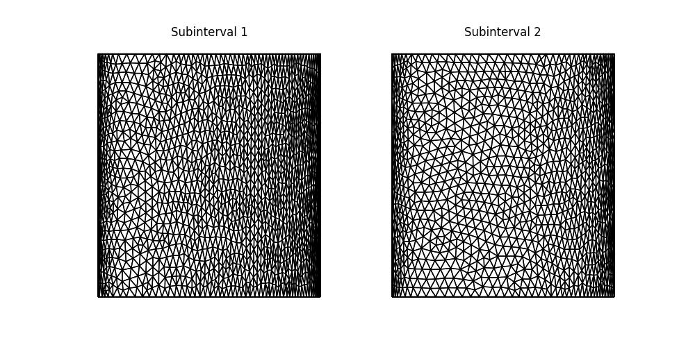
Recall that the Burgers problem is quasi-1D, since the analytical solution varies in the \(x\)-direction, but is constant in the \(y\)-direction. As such, we can affort to have lower resolution in the \(y\)-direction in adapted meshes. That this occurs is clear from the plots above. The solution moves to the right, becoming more densely distributed near to the right-hand boundary. This can be seen by comparing the second mesh against the first.
Exercise
In this demo, we obtain a Hessian metric by recovering Hessians of the two velocity components and combining them using metric intersection. Try out other approaches, such as combining using metric addition and recovering a single Hessian of the speed (i.e., the square root of the dot product of the velocity with itself).
This demo can also be accessed as a Python script.