Goal-oriented mesh adaptation for a 2D steady-state problem

In the previous demo, we applied Hessian-based mesh adaptation to the “point discharge with diffusion” steady-state 2D test case. Here, we combine the goal-oriented error estimation approach from another previous demo to provide the first exposition of goal-oriented mesh adaptation in these demos.

We copy over the setup as before. The only difference is that we import from goalie_adjoint rather than goalie.

import matplotlib.colors as mcolors
import matplotlib.pyplot as plt
from animate.adapt import adapt
from animate.metric import RiemannianMetric
from firedrake import *
from matplotlib import ticker

from goalie_adjoint import *

field_names = ["c"]


def get_function_spaces(mesh):
    return {"c": FunctionSpace(mesh, "CG", 1)}


def source(mesh):
    x, y = SpatialCoordinate(mesh)
    x0, y0, r = 2, 5, 0.05606388
    return 100.0 * exp(-((x - x0) ** 2 + (y - y0) ** 2) / r**2)


def get_form(mesh_seq):
    def form(index):
        c = mesh_seq.fields["c"]
        function_space = mesh_seq.function_spaces["c"][index]
        h = CellSize(mesh_seq[index])
        S = source(mesh_seq[index])

        # Define constants
        R = FunctionSpace(mesh_seq[index], "R", 0)
        D = Function(R).assign(0.1)
        u_x = Function(R).assign(1.0)
        u_y = Function(R).assign(0.0)
        u = as_vector([u_x, u_y])

        # SUPG stabilisation parameter
        unorm = sqrt(dot(u, u))
        tau = 0.5 * h / unorm
        tau = min_value(tau, unorm * h / (6 * D))

        # Setup variational problem
        psi = TestFunction(function_space)
        psi = psi + tau * dot(u, grad(psi))
        F = (
            dot(u, grad(c)) * psi * dx
            + inner(D * grad(c), grad(psi)) * dx
            - S * psi * dx
        )
        return {"c": F}

    return form


def get_solver(mesh_seq):
    def solver(index):
        function_space = mesh_seq.function_spaces["c"][index]
        c = mesh_seq.fields["c"]

        # Setup variational problem
        F = mesh_seq.form(index)["c"]
        bc = DirichletBC(function_space, 0, 1)

        solve(F == 0, c, bcs=bc, ad_block_tag="c")
        yield

    return solver


def get_qoi(mesh_seq, index):
    def qoi():
        c = mesh_seq.fields["c"]
        x, y = SpatialCoordinate(mesh_seq[index])
        xr, yr, rr = 20, 7.5, 0.5
        kernel = conditional((x - xr) ** 2 + (y - yr) ** 2 < rr**2, 1, 0)
        return kernel * c * dx

    return qoi

Since we want to do goal-oriented mesh adaptation, we use a GoalOrientedMeshSeq. In addition to the element count convergence criterion, we add another relative tolerance condition for the change in QoI value between iterations.

params = GoalOrientedMetricParameters(
    {
        "element_rtol": 0.005,
        "qoi_rtol": 0.005,
        "maxiter": 35,
    }
)

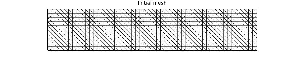
mesh = RectangleMesh(50, 10, 50, 10)
time_partition = TimeInstant(field_names)
mesh_seq = GoalOrientedMeshSeq(
    time_partition,
    mesh,
    get_function_spaces=get_function_spaces,
    get_form=get_form,
    get_solver=get_solver,
    get_qoi=get_qoi,
    qoi_type="steady",
    parameters=params,
)

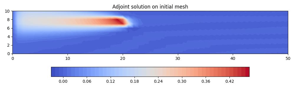
Let’s solve the adjoint problem on the initial mesh so that we can see what the corresponding solution looks like.

solutions = mesh_seq.solve_adjoint()
plot_kwargs = {"levels": 50, "figsize": (10, 3), "cmap": "coolwarm"}
interior_kw = {"linewidth": 0.5}
fig, axes, tcs = plot_snapshots(
    solutions,
    time_partition,
    "c",
    "adjoint",
    **plot_kwargs,
)
cbar = fig.colorbar(tcs[0][0], orientation="horizontal", pad=0.2)
axes.set_title("Adjoint solution on initial mesh")
fig.savefig("point_discharge2d-adjoint_init.jpg")
plt.close()

The adaptor takes a different form in this case, depending on adjoint solution data as well as forward solution data. For simplicity, we begin by using Goalie’s inbuilt isotropic metric function.

def adaptor(mesh_seq, solutions, indicators):
    # Deduce an isotropic metric from the error indicator field
    P1_ten = TensorFunctionSpace(mesh_seq[0], "CG", 1)
    metric = RiemannianMetric(P1_ten)
    metric.compute_isotropic_metric(indicators["c"][0][0])

    # Ramp the target metric complexity from 400 to 1000 over the first few iterations
    base, target, iteration = 400, 1000, mesh_seq.fp_iteration
    mp = {"dm_plex_metric_target_complexity": ramp_complexity(base, target, iteration)}
    metric.set_parameters(mp)

    # Normalise the metric according to the target complexity and then adapt the mesh
    metric.normalise()
    complexity = metric.complexity()
    mesh_seq[0] = adapt(mesh_seq[0], metric)
    num_dofs = mesh_seq.count_vertices()[0]
    num_elem = mesh_seq.count_elements()[0]
    pyrint(
        f"{iteration + 1:2d}, complexity: {complexity:4.0f}"
        f", dofs: {num_dofs:4d}, elements: {num_elem:4d}"
    )

    # Plot each intermediate adapted mesh
    fig, axes = plt.subplots(figsize=(10, 2))
    mesh_seq.plot(fig=fig, axes=axes, interior_kw=interior_kw)
    axes.set_title(f"Mesh at iteration {iteration + 1}")
    fig.savefig(f"point_discharge2d-iso_go_mesh{iteration + 1}.jpg")
    plt.close()

    # Plot error indicator on intermediate meshes
    plot_kwargs["norm"] = mcolors.LogNorm()
    plot_kwargs["locator"] = ticker.LogLocator()
    fig, axes, tcs = plot_indicator_snapshots(
        indicators, time_partition, "c", **plot_kwargs
    )
    axes.set_title(f"Indicator at iteration {mesh_seq.fp_iteration + 1}")
    fig.colorbar(tcs[0][0], orientation="horizontal", pad=0.2)
    fig.savefig(f"point_discharge2d-iso_go_indicator{mesh_seq.fp_iteration + 1}.jpg")
    plt.close()

    # Check whether the target complexity has been (approximately) reached. If not,
    # return ``True`` to indicate that convergence checks should be skipped until the
    # next fixed point iteration.
    continue_unconditionally = complexity < 0.95 * target
    return [continue_unconditionally]

With the adaptor function defined, we can call the fixed point iteration method. Note that, in addition to solving the forward problem, this version of the fixed point iteration method solves the adjoint problem, as well as solving the forward problem again on a globally uniformly refined mesh. The latter is particularly expensive, so we should expect the computation to take more time.

solutions, indicators = mesh_seq.fixed_point_iteration(adaptor)

This time, we find that the fixed point iteration converges in five iterations. Convergence is reached because the relative change in QoI is found to be smaller than the default tolerance.

 1, complexity:  371, dofs:  526, elements:  988
 2, complexity:  588, dofs:  729, elements: 1392
 3, complexity:  785, dofs:  916, elements: 1754
 4, complexity:  982, dofs: 1171, elements: 2264
 5, complexity:  984, dofs: 1151, elements: 2225
 6, complexity:  988, dofs: 1174, elements: 2269
 7, complexity:  985, dofs: 1170, elements: 2264
Element count converged after 7 iterations under relative tolerance 0.005.

fig, axes = plt.subplots(figsize=(10, 2))
mesh_seq.plot(fig=fig, axes=axes, interior_kw=interior_kw)
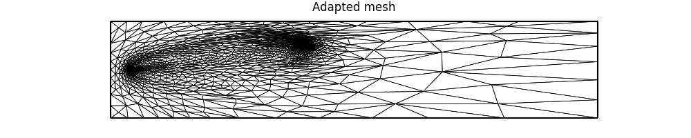
axes.set_title("Adapted mesh")
fig.savefig("point_discharge2d-iso_go_mesh.jpg")
plt.close()

plot_kwargs = {"levels": 50, "figsize": (10, 3), "cmap": "coolwarm"}
fig, axes, tcs = plot_snapshots(
    solutions,
    time_partition,
    "c",
    "forward",
    **plot_kwargs,
)
fig.colorbar(tcs[0][0], orientation="horizontal", pad=0.2)
axes.set_title("Forward solution on adapted mesh")
fig.savefig("point_discharge2d-forward_iso_go_adapted.jpg")
plt.close()

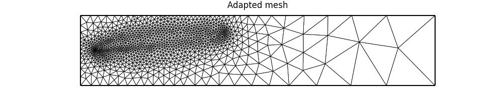
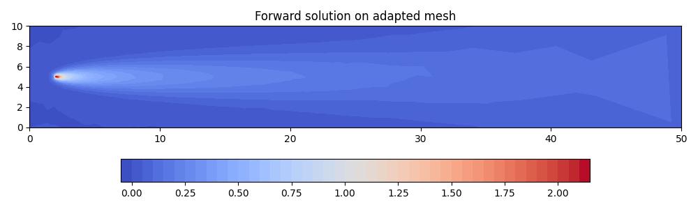
Looking at the final adapted mesh, we can make a few observations. Firstly, the mesh elements are indeed isotropic. Secondly, there is clearly increased resolution surrounding the point source, as well as the “receiver region” which the QoI integrates over. There is also a band of increased resolution between these two regions. Finally, the mesh has low resolution downstream of the receiver region. This is to be expected because we have an advection-dominated problem, so the QoI value is independent of the dynamics there.

Goalie also provides drivers for anisotropic goal-oriented mesh adaptation. Here, we consider the anisotropic_dwr_metric driver. (See documentation for details.) To use it, we just need to define a different adaptor function. The same error indicator is used as for the isotropic approach. In addition, the Hessian of the forward solution is provided to give anisotropy to the metric.

For this driver, normalisation is handled differently than for isotropic_metric, where the normalise method is called after construction. In this case, the metric is already normalised within the call to anisotropic_dwr_metric, so this is not required.

def adaptor(mesh_seq, solutions, indicators):
    P1_ten = TensorFunctionSpace(mesh_seq[0], "CG", 1)

    # Recover the Hessian of the forward solution
    hessian = RiemannianMetric(P1_ten)
    hessian.compute_hessian(solutions["c"]["forward"][0][0])

    # Ramp the target metric complexity from 400 to 1000 over the first few iterations
    metric = RiemannianMetric(P1_ten)
    base, target, iteration = 400, 1000, mesh_seq.fp_iteration
    mp = {"dm_plex_metric_target_complexity": ramp_complexity(base, target, iteration)}
    metric.set_parameters(mp)

    # Deduce an anisotropic metric from the error indicator field and the Hessian
    metric.compute_anisotropic_dwr_metric(indicators["c"][0][0], hessian)
    complexity = metric.complexity()

    # Adapt the mesh
    mesh_seq[0] = adapt(mesh_seq[0], metric)
    num_dofs = mesh_seq.count_vertices()[0]
    num_elem = mesh_seq.count_elements()[0]
    pyrint(
        f"{iteration + 1:2d}, complexity: {complexity:4.0f}"
        f", dofs: {num_dofs:4d}, elements: {num_elem:4d}"
    )

    # Plot each intermediate adapted mesh
    fig, axes = plt.subplots(figsize=(10, 2))
    mesh_seq.plot(fig=fig, axes=axes, interior_kw=interior_kw)
    axes.set_title(f"Mesh at iteration {iteration + 1}")
    fig.savefig(f"point_discharge2d-aniso_go_mesh{iteration + 1}.jpg")
    plt.close()

    # Plot error indicator on intermediate meshes
    plot_kwargs["norm"] = mcolors.LogNorm()
    plot_kwargs["locator"] = ticker.LogLocator()
    fig, axes, tcs = plot_indicator_snapshots(
        indicators, time_partition, "c", **plot_kwargs
    )
    axes.set_title(f"Indicator at iteration {mesh_seq.fp_iteration + 1}")
    fig.colorbar(tcs[0][0], orientation="horizontal", pad=0.2)
    fig.savefig(f"point_discharge2d-aniso_go_indicator{mesh_seq.fp_iteration + 1}.jpg")
    plt.close()

    # Check whether the target complexity has been (approximately) reached. If not,
    # return ``True`` to indicate that convergence checks should be skipped until the
    # next fixed point iteration.
    continue_unconditionally = complexity < 0.95 * target
    return [continue_unconditionally]

To avoid confusion, we redefine the GoalOrientedMeshSeq object before using it.

mesh_seq = GoalOrientedMeshSeq(
    time_partition,
    mesh,
    get_function_spaces=get_function_spaces,
    get_form=get_form,
    get_solver=get_solver,
    get_qoi=get_qoi,
    qoi_type="steady",
    parameters=params,
)
solutions, indicators = mesh_seq.fixed_point_iteration(adaptor)

 1, complexity:  400, dofs:  542, elements: 1030
 2, complexity:  600, dofs:  749, elements: 1450
 3, complexity:  800, dofs:  977, elements: 1908
 4, complexity: 1000, dofs: 1204, elements: 2364
 5, complexity: 1000, dofs: 1275, elements: 2506
 6, complexity: 1000, dofs: 1254, elements: 2464
 7, complexity: 1000, dofs: 1315, elements: 2584
 8, complexity: 1000, dofs: 1281, elements: 2519
 9, complexity: 1000, dofs: 1351, elements: 2657
10, complexity: 1000, dofs: 1295, elements: 2546
11, complexity: 1000, dofs: 1283, elements: 2523
12, complexity: 1000, dofs: 1336, elements: 2628
13, complexity: 1000, dofs: 1309, elements: 2574
14, complexity: 1000, dofs: 1304, elements: 2564
Element count converged after 14 iterations under relative tolerance 0.005.

fig, axes = plt.subplots(figsize=(10, 2))
mesh_seq.plot(fig=fig, axes=axes, interior_kw=interior_kw)
axes.set_title("Adapted mesh")
fig.savefig("point_discharge2d-aniso_go_mesh.jpg")
plt.close()

plot_kwargs = {"levels": 50, "figsize": (10, 3), "cmap": "coolwarm"}
fig, axes, tcs = plot_snapshots(
    solutions,
    time_partition,
    "c",
    "forward",
    **plot_kwargs,
)
fig.colorbar(tcs[0][0], orientation="horizontal", pad=0.2)
axes.set_title("Forward solution on adapted mesh")
fig.savefig("point_discharge2d-forward_aniso_go_adapted.jpg")
plt.close()

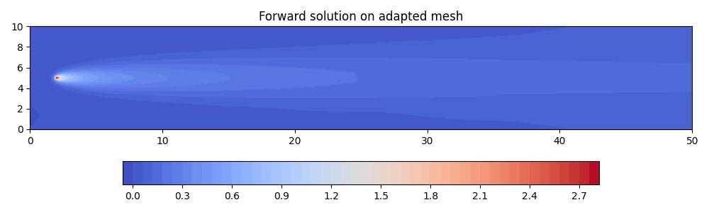
This time, the elements are clearly anisotropic. This anisotropy is inherited from the Hessian of the adjoint solution. There is still high resolution at the source and receiver, as well as coarse resolution downstream.

In the next demo, we consider mesh adaptation in the time-dependent case.

This demo can also be accessed as a Python script.