Point discharge with diffusion

Goalie has been developed primarily with time-dependent problems in mind, since the loop structures required to solve forward and adjoint problems and do goal-oriented error estimation and mesh adaptation are rather complex for such cases. However, it can also be used to solve steady-state problems.

Consider the same steady-state advection-diffusion test case as in the motivation for the Goalie manual: the “point discharge with diffusion” test case from [RCJ14]. In this test case, we solve

\[\begin{split}\left\{\begin{array}{rl} \mathbf u\cdot\nabla c - \nabla\cdot(D\nabla c) = S & \text{in}\:\Omega\\ c=0 & \text{on}\:\partial\Omega_{\mathrm{inflow}}\\ \nabla c\cdot\widehat{\mathbf n}=0 & \text{on}\:\partial\Omega\backslash\partial\Omega_{\mathrm{inflow}} \end{array}\right.,\end{split}\]

for a tracer concentration \(c\), with fluid velocity \(\mathbf u\), diffusion coefficient \(D\) and point source representation \(S\). The domain of interest is the rectangle \(\Omega = [0, 50] \times [0, 10]\).

As always, start by importing Firedrake and Goalie.

from firedrake import *

from goalie_adjoint import *

We solve the advection-diffusion problem in \(\mathbb P1\) space.

field_names = ["c"]


def get_function_spaces(mesh):
    return {"c": FunctionSpace(mesh, "CG", 1)}

Point sources are difficult to represent in numerical models. Here we follow [WBHP22] in using a Gaussian approximation. Let \((x_0,y_0)=(2,5)\) denote the point source location and \(r=0.05606388\) be a radius parameter, which has been calibrated so that the finite element approximation is as close as possible to the analytical solution, in some sense (see [WBHP22] for details).

def source(mesh):
    x, y = SpatialCoordinate(mesh)
    x0, y0, r = 2, 5, 0.05606388
    return 100.0 * exp(-((x - x0) ** 2 + (y - y0) ** 2) / r**2)

On its own, a \(\mathbb P1\) discretisation is unstable for this problem. Therefore, we include additional streamline upwind Petrov Galerkin (SUPG) stabilisation by modifying the test function \(\psi\) according to

\[\psi \mapsto \psi + \tau\mathbf u\cdot\nabla\psi,\]

with stabilisation parameter

\[\tau = \min\left(\frac{h}{2\|\mathbf u\|},\frac{h\|\mathbf u\|}{6D}\right),\]

where \(h\) measures cell size.

def get_form(mesh_seq):
    def form(index):
        c = mesh_seq.fields["c"]
        function_space = mesh_seq.function_spaces["c"][index]
        h = CellSize(mesh_seq[index])
        S = source(mesh_seq[index])

        # Define constants
        R = FunctionSpace(mesh_seq[index], "R", 0)
        D = Function(R).assign(0.1)
        u_x = Function(R).assign(1.0)
        u_y = Function(R).assign(0.0)
        u = as_vector([u_x, u_y])

        # SUPG stabilisation parameter
        unorm = sqrt(dot(u, u))
        tau = 0.5 * h / unorm
        tau = min_value(tau, unorm * h / (6 * D))

        # Setup variational problem
        psi = TestFunction(function_space)
        psi = psi + tau * dot(u, grad(psi))
        F = (
            dot(u, grad(c)) * psi * dx
            + inner(D * grad(c), grad(psi)) * dx
            - S * psi * dx
        )
        return {"c": F}

    return form

Note that mesh_seq.fields now returns a single Function object since the problem is steady, so there is no notion of a lagged solution, unlike in previous (time-dependent) demos. With these ingredients, we can now define the get_solver() method. Don’t forget to apply the corresponding ad_block_tag to the solve call.

def get_solver(mesh_seq):
    def solver(index):
        function_space = mesh_seq.function_spaces["c"][index]

        c = mesh_seq.fields["c"]

        # Setup variational problem
        F = mesh_seq.form(index)["c"]

        # Strongly enforce boundary conditions on the inflow, which is indexed by 1
        bc = DirichletBC(function_space, 0, 1)

        solve(F == 0, c, bcs=bc, ad_block_tag="c")
        yield

    return solver

For steady-state problems, we do not need to specify get_initial_condition() if the equation is linear. If the equation is nonlinear then this would provide an initial guess. By default, all components are initialised to zero.

As in the motivation for the manual, we consider a quantity of interest that integrates the tracer concentration over a circular “receiver” region. Since there is no time dependence, the QoI looks just like an "end_time" type QoI.

def get_qoi(mesh_seq, index):
    def qoi():
        c = mesh_seq.fields["c"]
        x, y = SpatialCoordinate(mesh_seq[index])
        xr, yr, rr = 20, 7.5, 0.5
        kernel = conditional((x - xr) ** 2 + (y - yr) ** 2 < rr**2, 1, 0)
        return kernel * c * dx

    return qoi

Finally, we can set up the problem. Instead of using a TimePartition, we use the subclass TimeInstant, whose only input is the field list.

mesh = RectangleMesh(200, 40, 50, 10)
time_partition = TimeInstant(field_names)

When creating the MeshSeq, we need to set the "qoi_type" to "steady".

mesh_seq = GoalOrientedMeshSeq(
    time_partition,
    mesh,
    get_function_spaces=get_function_spaces,
    get_form=get_form,
    get_solver=get_solver,
    get_qoi=get_qoi,
    qoi_type="steady",
)
solutions, indicators = mesh_seq.indicate_errors(
    enrichment_kwargs={"enrichment_method": "p"}
)

We can plot the solution fields and error indicators as follows.

import matplotlib.colors as mcolors
from matplotlib import ticker

plot_kwargs = {"levels": 50, "figsize": (10, 3), "cmap": "coolwarm"}
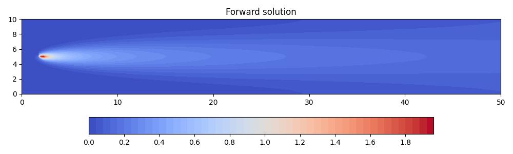
fig, axes, tcs = plot_snapshots(
    solutions, time_partition, "c", "forward", **plot_kwargs
)
fig.colorbar(tcs[0][0], orientation="horizontal", pad=0.2)
axes.set_title("Forward solution")
fig.savefig("point_discharge2d-forward.jpg")
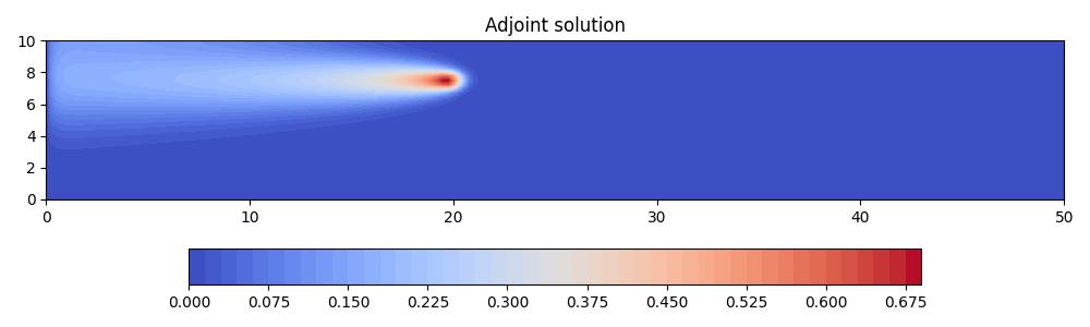
fig, axes, tcs = plot_snapshots(
    solutions, time_partition, "c", "adjoint", **plot_kwargs
)
fig.colorbar(tcs[0][0], orientation="horizontal", pad=0.2)
axes.set_title("Adjoint solution")
fig.savefig("point_discharge2d-adjoint.jpg")
plot_kwargs["norm"] = mcolors.LogNorm()
plot_kwargs["locator"] = ticker.LogLocator()
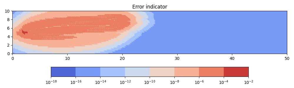
fig, axes, tcs = plot_indicator_snapshots(
    indicators, time_partition, "c", **plot_kwargs
)
cbar = fig.colorbar(tcs[0][0], orientation="horizontal", pad=0.2)
axes.set_title("Error indicator")
fig.savefig("point_discharge2d-indicator.jpg")

The forward solution is driven by a point source, which is advected from left to right and diffused uniformly in all directions.

The adjoint solution, on the other hand, is driven by a source term at the receiver and is advected from right to left. It is also diffused uniformly in all directions.

The resulting goal-oriented error indicator field is non-zero inbetween the source and receiver, implying that the largest contributions towards QoI error come from these parts of the domain. By contrast, the contributions from downstream regions are negligible.

In the next tutorial we will apply metric-based mesh adaptation to the point discharge test case considered here.

This tutorial can be dowloaded as a Python script.