Hessian-based mesh adaptation for a 2D steady-state problem

Previous demos have covered the fundamental time partition and mesh sequence objects of Goalie, using them to solve PDEs over multiple meshes and perform goal-oriented error estimation. Here, we demonstrate how to use them for Hessian-based mesh adaptation for a steady-state problem in 2D.

It is recommended that you read the documentation on metric-based mesh adaptation before progressing with this demo.

In addition to importing from Firedrake and Goalie, we also import the mesh adaptation functionality from Firedrake, which can be found in firedrake.meshadapt.

from animate.adapt import adapt
from animate.metric import RiemannianMetric
from firedrake import *

from goalie import *

We again consider the “point discharge with diffusion” test case from the previous demo, approximating the tracer concentration \(c\) in \(\mathbb P1\) space.

field_names = ["c"]


def get_function_spaces(mesh):
    return {"c": FunctionSpace(mesh, "CG", 1)}


def source(mesh):
    x, y = SpatialCoordinate(mesh)
    x0, y0, r = 2, 5, 0.05606388
    return 100.0 * exp(-((x - x0) ** 2 + (y - y0) ** 2) / r**2)


def get_form(mesh_seq):
    def form(index):
        c = mesh_seq.fields["c"]
        function_space = mesh_seq.function_spaces["c"][index]
        h = CellSize(mesh_seq[index])
        S = source(mesh_seq[index])

        # Define constants
        R = FunctionSpace(mesh_seq[index], "R", 0)
        D = Function(R).assign(0.1)
        u_x = Function(R).assign(1.0)
        u_y = Function(R).assign(0.0)
        u = as_vector([u_x, u_y])

        # SUPG stabilisation parameter
        unorm = sqrt(dot(u, u))
        tau = 0.5 * h / unorm
        tau = min_value(tau, unorm * h / (6 * D))

        # Setup variational problem
        psi = TestFunction(function_space)
        psi = psi + tau * dot(u, grad(psi))
        F = (
            dot(u, grad(c)) * psi * dx
            + inner(D * grad(c), grad(psi)) * dx
            - S * psi * dx
        )
        return {"c": F}

    return form


def get_solver(mesh_seq):
    def solver(index):
        function_space = mesh_seq.function_spaces["c"][index]
        c = mesh_seq.fields["c"]

        # Setup variational problem
        F = mesh_seq.form(index)["c"]
        bc = DirichletBC(function_space, 0, 1)

        solve(F == 0, c, bcs=bc, ad_block_tag="c")
        yield

    return solver

Take a relatively coarse initial mesh, a TimeInstant (since we have a steady-state problem), and put everything together in a MeshSeq. For this demo, we also create a MetricParameters object and set the element_rtol parameter to 0.005. This means that the fixed point iteration will terminate if the element count changes by less than 0.5% between iterations. As standard, we allow 35 iterations before establishing that the iteration is not going to converge. To cut down the cost of the regresssion tests, we just use three iterations instead.

params = MetricParameters(
    {
        "element_rtol": 0.005,
        "maxiter": 35,
    }
)

mesh = RectangleMesh(50, 10, 50, 10)
time_partition = TimeInstant(field_names)
mesh_seq = MeshSeq(
    time_partition,
    mesh,
    get_function_spaces=get_function_spaces,
    get_form=get_form,
    get_solver=get_solver,
    parameters=params,
)

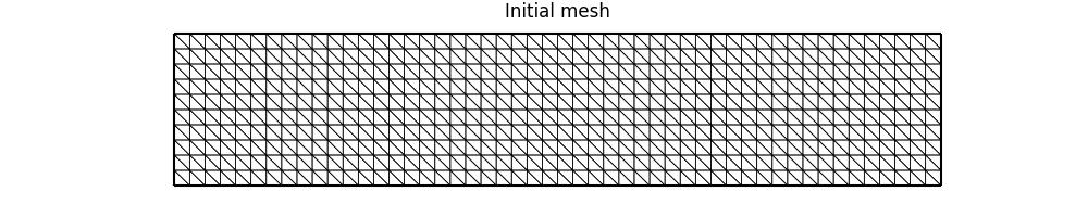
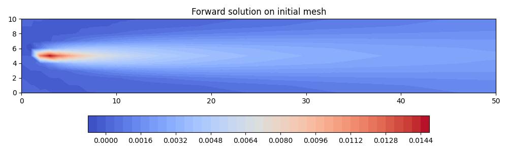
Give the initial mesh, we can plot it, solve the PDE on it, and plot the resulting solution field.

import matplotlib.pyplot as plt

fig, axes = plt.subplots(figsize=(10, 2))
interior_kw = {"linewidth": 0.5}
mesh_seq.plot(fig=fig, axes=axes, interior_kw=interior_kw)
axes.set_title("Initial mesh")
fig.savefig("point_discharge2d-mesh0.jpg")
plt.close()

solutions = mesh_seq.solve_forward()

plot_kwargs = {"levels": 50, "figsize": (10, 3), "cmap": "coolwarm"}
fig, axes, tcs = plot_snapshots(
    solutions,
    time_partition,
    "c",
    "forward",
    **plot_kwargs,
)
cbar = fig.colorbar(tcs[0][0], orientation="horizontal", pad=0.2)
axes.set_title("Forward solution on initial mesh")
fig.savefig("point_discharge2d-forward_init.jpg")
plt.close()

In order to perform metric-based mesh adaptation, we need to tell the mesh sequence how to define metrics and adapt its meshes. Since we have a steady-state problem, there is only ever one mesh, one solution field, and one metric, so this simplifies things significantly.

For this first example, we compute a metric by recovering the Hessian of the approximate solution field, and scaling it according to a desired metric complexity using \(L^p\) normalisation. The normalised metric is used to adapt the mesh, which we print the obtained metric complexity and DoF count of the adapted mesh. Since the solution is sought in \(\mathbb P1\) space, the DoF count is just the vertex count.

def adaptor(mesh_seq, solutions):
    c = solutions["c"]["forward"][0][0]

    # Define the Riemannian metric
    P1_tensor = TensorFunctionSpace(mesh_seq[0], "CG", 1)
    metric = RiemannianMetric(P1_tensor)

    # Recover the Hessian of the current solution
    metric.compute_hessian(c)

    # Ramp the target metric complexity from 400 to 1000 over the first few iterations
    base, target, iteration = 400, 1000, mesh_seq.fp_iteration
    mp = {"dm_plex_metric_target_complexity": ramp_complexity(base, target, iteration)}
    metric.set_parameters(mp)

    # Normalise the metric according to the target complexity and then adapt the mesh
    metric.normalise()
    complexity = metric.complexity()
    mesh_seq[0] = adapt(mesh_seq[0], metric)
    num_dofs = mesh_seq.count_vertices()[0]
    num_elem = mesh_seq.count_elements()[0]
    pyrint(
        f"{iteration + 1:2d}, complexity: {complexity:4.0f}"
        f", dofs: {num_dofs:4d}, elements: {num_elem:4d}"
    )

    # Plot each intermediate adapted mesh
    fig, axes = plt.subplots(figsize=(10, 2))
    mesh_seq.plot(fig=fig, axes=axes, interior_kw=interior_kw)
    axes.set_title(f"Mesh at iteration {iteration + 1}")
    fig.savefig(f"point_discharge2d-hessian_mesh{iteration + 1}.jpg")
    plt.close()

    # Check whether the target complexity has been (approximately) reached. If not,
    # return ``True`` to indicate that convergence checks should be skipped until the
    # next fixed point iteration.
    continue_unconditionally = complexity < 0.95 * target
    return [continue_unconditionally]

With the adaptor function defined, we can call the fixed point iteration method, which iteratively solves the PDE and calls the adaptor until one of the convergence criteria are met.

solutions = mesh_seq.fixed_point_iteration(adaptor)

Mesh adaptation often gives slightly different results on difference machines. However, the output should look something like

 1, complexity:  433, dofs:  618, elements: 1161
 2, complexity:  630, dofs:  898, elements: 1725
 3, complexity:  825, dofs: 1128, elements: 2180
 4, complexity: 1023, dofs: 1336, elements: 2592
 5, complexity: 1020, dofs: 1354, elements: 2629
 6, complexity: 1022, dofs: 1362, elements: 2643
 7, complexity: 1022, dofs: 1356, elements: 2635
Element count converged after 7 iterations under relative tolerance 0.005.

We can plot the final mesh and the corresponding solution as follows.

fig, axes = plt.subplots(figsize=(10, 2))
mesh_seq.plot(fig=fig, axes=axes, interior_kw=interior_kw)
axes.set_title("Adapted mesh")
fig.savefig("point_discharge2d-hessian_mesh.jpg")
plt.close()

fig, axes, tcs = plot_snapshots(
    solutions,
    time_partition,
    "c",
    "forward",
    **plot_kwargs,
)
cbar = fig.colorbar(tcs[0][0], orientation="horizontal", pad=0.2)
axes.set_title("Forward solution on adapted mesh")
fig.savefig("point_discharge2d-forward_hessian_adapted.jpg")
plt.close()

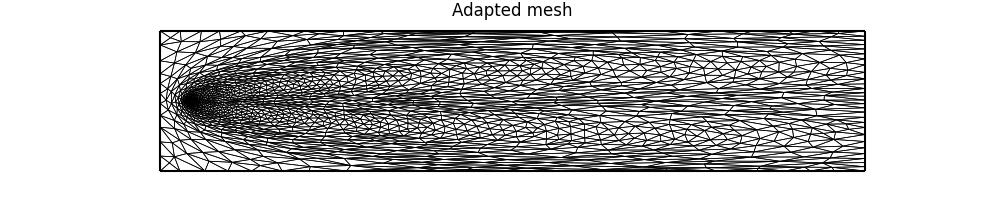
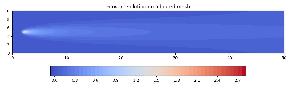
Notice how the adapted mesh has increased resolution in the regions of highest curvature in the solution field. Moreover, it is anisotropic, with the orientation of anisotropic elements aligned with the contours of the solution field.

In the next demo, we consider the same problem again, but using goal-oriented mesh adaptation.

This demo can also be accessed as a Python script.