Burgers equation on a sequence of meshes

This demo shows how to solve the Firedrake Burgers equation demo on a sequence of meshes using Goalie. The PDE

\[ \begin{align}\begin{aligned}\begin{split}\frac{\partial\mathbf u}{\partial t} + (\mathbf u\cdot\nabla)\mathbf u - \nu\nabla^2\mathbf u = \boldsymbol0 \quad\text{in}\quad \Omega\\\end{split}\\(\widehat{\mathbf n}\cdot\nabla)\mathbf u = \boldsymbol0 \quad\text{on}\quad \partial\Omega\end{aligned}\end{align} \]

is solved on two meshes of the unit square, \(\Omega = [0, 1]^2\). The forward solution is initialised as a sine wave and is nonlinearly advected to the right hand side. See the Firedrake demo for details on the discretisation used.

from firedrake import *

from goalie import *

In this problem, we have a single prognostic variable, \(\mathbf u\). Its name is recorded in a list of field names.

field_names = ["u"]

For each such field, we need to be able to specify how to build a FunctionSpace, given some mesh. Since there could be more than one field, function spaces are given as a dictionary, indexed by the prognostic solution field names.

def get_function_spaces(mesh):
    return {"u": VectorFunctionSpace(mesh, "CG", 2)}

In order to solve PDEs using the finite element method, we require a weak form. For this, Goalie requires a function that maps the MeshSeq index and a dictionary of solution data to the form. The form should be returned inside its own dictionary, with an entry for each equation being solved for.

The solution Functions are automatically built on the function spaces given by the get_function_spaces() function and are accessed via the fields attribute of the MeshSeq. This attribute provides a dictionary of tuples containing the current and lagged solutions for each field. Similarly, timestepping information associated with a given subinterval can be accessed via the TimePartition attribute of the MeshSeq. For technical reasons, we need to create a Function in the ‘R’ space (of real numbers) to hold constants.

def get_form(mesh_seq):
    def form(index):
        # Get the current and lagged solutions
        u, u_ = mesh_seq.fields["u"]

        # Define constants
        R = FunctionSpace(mesh_seq[index], "R", 0)
        dt = Function(R).assign(mesh_seq.time_partition.timesteps[index])
        nu = Function(R).assign(0.0001)

        # Setup variational problem
        v = TestFunction(u.function_space())
        F = (
            inner((u - u_) / dt, v) * dx
            + inner(dot(u, nabla_grad(u)), v) * dx
            + nu * inner(grad(u), grad(v)) * dx
        )
        return {"u": F}

    return form

We have a weak form. The dictionary usage may seem cumbersome when applied to such a simple problem, but it comes in handy when solving adjoint problems associated with coupled systems of equations.

In order to solve the PDE, we need to choose a time integration routine and solver parameters for the underlying linear and nonlinear systems. This is achieved below by using a function solver() whose input is the MeshSeq index. As noted above, the solution Functions are automatically initialised and accessed via the fields attribute of the MeshSeq. The lagged solution is assigned the initial condition for the current subinterval index. For the \(0^{th}\) index, this will be provided by the initial conditions, otherwise it will be transferred from the previous mesh in the sequence.

The function should return a generator that yields the solution at each timestep, so that Goalie can efficiently track the solution history. This is done by using the yield statement before progressing to the next timestep.

def get_solver(mesh_seq):
    def solver(index):
        # Get the current and lagged solutions
        u, u_ = mesh_seq.fields["u"]

        # Define form
        F = mesh_seq.form(index)["u"]

        # Time integrate from t_start to t_end
        tp = mesh_seq.time_partition
        t_start, t_end = tp.subintervals[index]
        dt = tp.timesteps[index]
        t = t_start
        while t < t_end - 1.0e-05:
            solve(F == 0, u)
            yield

            u_.assign(u)
            t += dt

    return solver

Goalie also requires a function for generating an initial condition from the function space defined on the \(0^{th}\) mesh.

def get_initial_condition(mesh_seq):
    fs = mesh_seq.function_spaces["u"][0]
    x, y = SpatialCoordinate(mesh_seq[0])
    return {"u": assemble(interpolate(as_vector([sin(pi * x), 0]), fs))}

Now that we have the above functions defined, we move onto the concrete parts of the solver. To begin with, we require a sequence of meshes, simulation end time and a timestep.

n = 32
meshes = [
    UnitSquareMesh(n, n),
    UnitSquareMesh(n, n),
]
end_time = 0.5
dt = 1 / n

These can be used to create a TimePartition for the problem with two subintervals.

num_subintervals = len(meshes)
time_partition = TimePartition(
    end_time,
    num_subintervals,
    dt,
    field_names,
    num_timesteps_per_export=2,
)

Finally, we are able to construct a MeshSeq and solve Burgers equation over the meshes in sequence.

mesh_seq = MeshSeq(
    time_partition,
    meshes,
    get_function_spaces=get_function_spaces,
    get_initial_condition=get_initial_condition,
    get_form=get_form,
    get_solver=get_solver,
)
solutions = mesh_seq.solve_forward()

During the solve_forward() call, the solver that was provided is applied on the first subinterval. The forward solution at the end of that subinterval is transferred to the mesh associated with the second subinterval and used as an initial condition for the same solver applied again there. Goalie uses a conservative interpolation operator to transfer solution data between the two meshes. In this example, the meshes (and hence function spaces) are identical so the projection operation will in fact be the identity.

The output is a nested dictionary of solution data, indexed by solution type ("forward" or "forward_old") and then field name (here "u"). The contents of the inner dictionaries are lists containing lists of solution Functions, indexed first by subinterval and then by timestep. That is, solutions["forward"]["u"][i][j] contains the forward solution associated with field "u" at the j-th timestep of subinterval i. Similarly, solutions["forward_old"]["u"][i][j] contains the forward solution from the timestep prior.

For the purposes of this demo, we plot the solution at each exported timestep using the plotting driver function plot_snapshots().

fig, axes, tcs = plot_snapshots(
    solutions, time_partition, "u", "forward", levels=np.linspace(0, 1, 9)
)
fig.savefig("burgers.jpg")

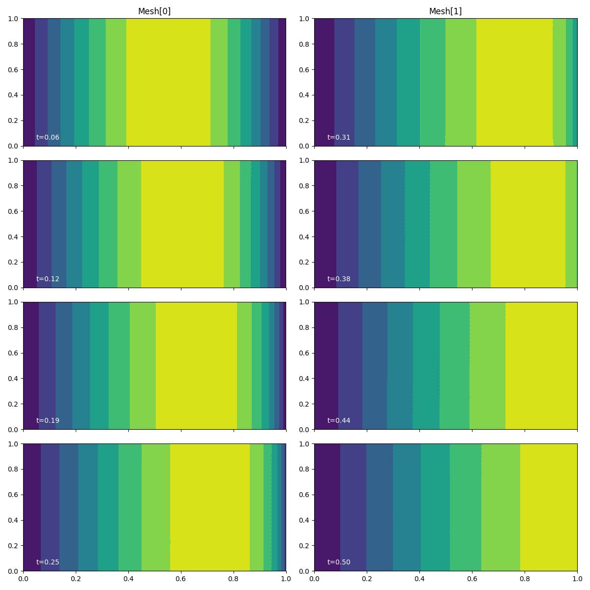
We see that the initial sinusoid is nonlinearly advected Eastwards.

In the next demo, we use Goalie to automatically solve the adjoint problem associated with Burgers equation.

This demo can also be accessed as a Python script.