Adjoint of Burgers equation

This demo solves the same problem as the previous one, but making use of dolfin-adjoint’s automatic differentiation functionality in order to automatically form and solve discrete adjoint problems.

We always begin by importing Goalie. Adjoint mode is used so that we have access to the AdjointMeshSeq class.

from firedrake import *

from goalie_adjoint import *

For ease, the list of field names and functions for obtaining the function spaces, forms, solvers, and initial conditions are redefined as in the previous demo. The only difference is that now we are solving the adjoint problem, which requires that the PDE solve is labelled with an ad_block_tag that matches the corresponding prognostic variable name.

field_names = ["u"]


def get_function_spaces(mesh):
    return {"u": VectorFunctionSpace(mesh, "CG", 2)}


def get_form(mesh_seq):
    def form(index):
        u, u_ = mesh_seq.fields["u"]

        # Define constants
        R = FunctionSpace(mesh_seq[index], "R", 0)
        dt = Function(R).assign(mesh_seq.time_partition.timesteps[index])
        nu = Function(R).assign(0.0001)

        # Setup variational problem
        v = TestFunction(u.function_space())
        F = (
            inner((u - u_) / dt, v) * dx
            + inner(dot(u, nabla_grad(u)), v) * dx
            + nu * inner(grad(u), grad(v)) * dx
        )
        return {"u": F}

    return form


def get_solver(mesh_seq):
    def solver(index):
        u, u_ = mesh_seq.fields["u"]

        # Define form
        F = mesh_seq.form(index)["u"]

        # Time integrate from t_start to t_end
        tp = mesh_seq.time_partition
        t_start, t_end = tp.subintervals[index]
        dt = tp.timesteps[index]
        t = t_start
        while t < t_end - 1.0e-05:
            solve(F == 0, u, ad_block_tag="u")  # Note the ad_block_tag
            yield

            u_.assign(u)
            t += dt

    return solver


def get_initial_condition(mesh_seq):
    fs = mesh_seq.function_spaces["u"][0]
    x, y = SpatialCoordinate(mesh_seq[0])
    return {"u": assemble(interpolate(as_vector([sin(pi * x), 0]), fs))}

In line with the firedrake-adjoint demo, we choose the QoI

\[J(u) = \int_0^1 \mathbf u(1,y,t_{\mathrm{end}}) \cdot \mathbf u(1,y,t_{\mathrm{end}})\;\mathrm dy,\]

which integrates the square of the solution \(\mathbf u(x,y,t)\) at the final time over the right hand boundary.

def get_qoi(mesh_seq, i):
    def end_time_qoi():
        u = mesh_seq.fields["u"][0]
        return inner(u, u) * ds(2)

    return end_time_qoi

Now that we have the above functions defined, we move onto the concrete parts of the solver, which mimic the original demo.

n = 32
mesh = UnitSquareMesh(n, n)
end_time = 0.5
dt = 1 / n

Another requirement to solve the adjoint problem using Goalie is a TimePartition. In our case, there is a single mesh, so the partition is trivial and we can use the TimeInterval constructor.

time_partition = TimeInterval(end_time, dt, field_names, num_timesteps_per_export=2)

Finally, we are able to construct an AdjointMeshSeq and thereby call its solve_adjoint() method. This computes the QoI value and returns a dictionary of solutions for the forward and adjoint problems.

mesh_seq = AdjointMeshSeq(
    time_partition,
    mesh,
    get_function_spaces=get_function_spaces,
    get_initial_condition=get_initial_condition,
    get_form=get_form,
    get_solver=get_solver,
    get_qoi=get_qoi,
    qoi_type="end_time",
)
solutions = mesh_seq.solve_adjoint()

The solution dictionary is similar to solve_forward(), except there are keys "adjoint" and "adjoint_next", in addition to "forward", "forward_old". For a given subinterval i and timestep index j, solutions["adjoint"]["u"][i][j] contains the adjoint solution associated with field "u" at that timestep, whilst solutions["adjoint_next"]["u"][i][j] contains the adjoint solution from the next timestep (with the arrow of time going forwards, as usual). Adjoint equations are solved backwards in time, so this is effectively the “lagged” adjoint solution, in the same way that "forward_old" corresponds to the “lagged” forward solution.

Finally, we plot the adjoint solution at each exported timestep by looping over solutions['adjoint']. This can also be achieved using the plotting driver function plot_snapshots.

fig, axes, tcs = plot_snapshots(
    solutions, time_partition, "u", "adjoint", levels=np.linspace(0, 0.8, 9)
)
fig.savefig("burgers1-end_time.jpg")

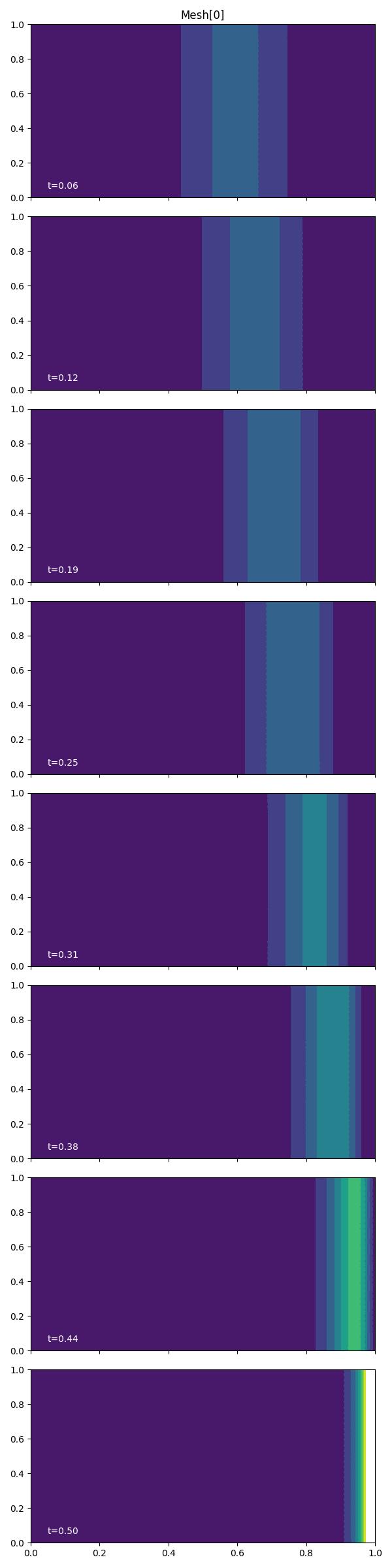
Since the arrow of time reverses for the adjoint problem, the plots should be read from bottom to top. The QoI acts as an impulse at the final time, which propagates in the opposite direction than information flows in the forward problem.

In the next demo, we solve the same problem on two subintervals and check that the results match.

This demo can also be accessed as a Python script.