Adjoint Burgers equation on two meshes

This demo solves the same adjoint problem as the previous one, but now using two subintervals. There is still no error estimation or mesh adaptation; the same mesh is used in each case to verify that the framework works.

Again, begin by importing Goalie with adjoint mode activated.

from firedrake import *

from goalie_adjoint import *

set_log_level(DEBUG)

Redefine the field_names variable from the previous demo, as well as all the getter functions.

field_names = ["u"]


def get_function_spaces(mesh):
    return {"u": VectorFunctionSpace(mesh, "CG", 2)}


def get_form(mesh_seq):
    def form(index):
        u, u_ = mesh_seq.fields["u"]

        # Define constants
        R = FunctionSpace(mesh_seq[index], "R", 0)
        dt = Function(R).assign(mesh_seq.time_partition.timesteps[index])
        nu = Function(R).assign(0.0001)

        # Setup variational problem
        v = TestFunction(u.function_space())
        F = (
            inner((u - u_) / dt, v) * dx
            + inner(dot(u, nabla_grad(u)), v) * dx
            + nu * inner(grad(u), grad(v)) * dx
        )
        return {"u": F}

    return form


def get_solver(mesh_seq):
    def solver(index):
        u, u_ = mesh_seq.fields["u"]

        # Define form
        F = mesh_seq.form(index)["u"]

        # Time integrate from t_start to t_end
        tp = mesh_seq.time_partition
        t_start, t_end = tp.subintervals[index]
        dt = tp.timesteps[index]
        t = t_start
        while t < t_end - 1.0e-05:
            solve(F == 0, u, ad_block_tag="u")
            yield

            u_.assign(u)
            t += dt

    return solver


def get_initial_condition(mesh_seq):
    fs = mesh_seq.function_spaces["u"][0]
    x, y = SpatialCoordinate(mesh_seq[0])
    return {"u": assemble(interpolate(as_vector([sin(pi * x), 0]), fs))}


def get_qoi(mesh_seq, i):
    def end_time_qoi():
        u = mesh_seq.fields["u"][0]
        return inner(u, u) * ds(2)

    return end_time_qoi

The solver, initial condition and QoI may be imported from the previous demo. The same basic setup is used. The only difference is that the MeshSeq contains two meshes.

n = 32
meshes = [UnitSquareMesh(n, n, diagonal="left"), UnitSquareMesh(n, n, diagonal="left")]
end_time = 0.5
dt = 1 / n

This time, the TimePartition is defined on two subintervals.

num_subintervals = len(meshes)
time_partition = TimePartition(
    end_time,
    num_subintervals,
    dt,
    field_names,
    num_timesteps_per_export=2,
)
mesh_seq = AdjointMeshSeq(
    time_partition,
    meshes,
    get_function_spaces=get_function_spaces,
    get_initial_condition=get_initial_condition,
    get_form=get_form,
    get_solver=get_solver,
    get_qoi=get_qoi,
    qoi_type="end_time",
)
solutions = mesh_seq.solve_adjoint()

Recall that solve_forward() runs the solver on each subinterval and uses conservative projection to transfer inbetween. This also happens in the forward pass of solve_adjoint(), but is followed by running the adjoint of the solver on each subinterval in reverse. The adjoint of the conservative projection operator is applied to transfer adjoint solution data between meshes in this case. If you think about the matrix representation of a projection operator then this effectively means taking the transpose. Again, the meshes (and hence function spaces) are identical, so the transfer is just the identity.

Snapshots of the adjoint solution are again plotted using the plot_snapshots() utility function.

fig, axes, tcs = plot_snapshots(
    solutions, time_partition, "u", "adjoint", levels=np.linspace(0, 0.8, 9)
)
fig.savefig("burgers2-end_time.jpg")

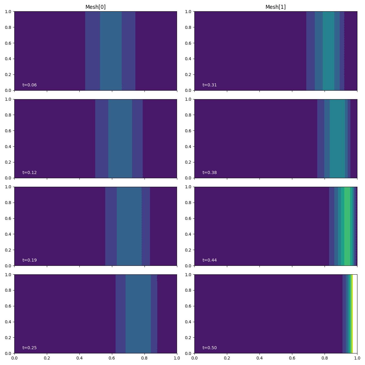
The adjoint solution fields at each time level appear to match those due to the previous demo at each timestep. That they actually do coincide is checked in Goalie’s test suite.

Exercise

Note that the keyword argument diagonal="left" was passed to the UnitSquareMesh constructor in this example, defining which way the diagonal lines in the uniform mesh should go. Instead of having both function spaces defined on this mesh, try defining the second one in a \(\mathbb P2\) space defined on a different mesh which is constructed with diagonal="right". How does the adjoint solution change when the solution is trasferred between different meshes? In this case, the mesh-to-mesh transfer operations will no longer simply be identities.

In the next demo, we solve the same problem but with a QoI involving an integral in time, as well as space.

This demo can also be accessed as a Python script.