Adjoint Burgers equation with a time integrated QoI

So far, we only considered a quantity of interest corresponding to a spatial integral at the end time. For some problems, it is more suitable to have a QoI which integrates in time as well as space.

Begin by importing from Goalie and the first Burgers demo.

from firedrake import *

from goalie_adjoint import *

Redefine the get_initial_condition, get_function_spaces, and get_form functions as in the first Burgers demo.

def get_function_spaces(mesh):
    return {"u": VectorFunctionSpace(mesh, "CG", 2)}


def get_form(mesh_seq):
    def form(index):
        u, u_ = mesh_seq.fields["u"]

        # Define constants
        R = FunctionSpace(mesh_seq[index], "R", 0)
        dt = Function(R).assign(mesh_seq.time_partition.timesteps[index])
        nu = Function(R).assign(0.0001)

        # Setup variational problem
        v = TestFunction(u.function_space())
        F = (
            inner((u - u_) / dt, v) * dx
            + inner(dot(u, nabla_grad(u)), v) * dx
            + nu * inner(grad(u), grad(v)) * dx
        )
        return {"u": F}

    return form


def get_initial_condition(mesh_seq):
    fs = mesh_seq.function_spaces["u"][0]
    x, y = SpatialCoordinate(mesh_seq[0])
    return {"u": assemble(interpolate(as_vector([sin(pi * x), 0]), fs))}

The solver needs to be modified slightly in order to take account of time dependent QoIs. The Burgers solver uses backward Euler timestepping. The corresponding quadrature routine is like the midpoint rule, but takes the value from the next timestep, rather than the average between that and the current value. As such, the QoI may be computed by simply incrementing the J attribute of the AdjointMeshSeq as follows.

def get_solver(mesh_seq):
    def solver(index):
        u, u_ = mesh_seq.fields["u"]

        # Define form
        F = mesh_seq.form(index)["u"]

        # Time integrate from t_start to t_end
        t_start, t_end = mesh_seq.subintervals[index]
        dt = mesh_seq.time_partition.timesteps[index]
        t = t_start
        qoi = mesh_seq.get_qoi(index)
        while t < t_end - 1.0e-05:
            solve(F == 0, u, ad_block_tag="u")
            mesh_seq.J += qoi(t)
            yield

            u_.assign(u)
            t += dt

    return solver

The QoI is effectively just a time-integrated version of the one previously seen.

\[J(u) = \int_0^{T_{\mathrm{end}}} \int_0^1 \mathbf u(1,y,t) \cdot \mathbf u(1,y,t) \;\mathrm dy\;\mathrm dt.\]

Note that in this case we multiply by the timestep. It is wrapped in a Function from ‘R’ space to avoid recompilation if the value is changed.

def get_qoi(mesh_seq, i):
    R = FunctionSpace(mesh_seq[i], "R", 0)
    dt = Function(R).assign(mesh_seq.time_partition.timesteps[i])

    def time_integrated_qoi(t):
        u = mesh_seq.fields["u"][0]
        return dt * inner(u, u) * ds(2)

    return time_integrated_qoi

We use the same mesh setup as in the previous demo and the same time partitioning, except that we export every timestep rather than every other timestep.

n = 32
meshes = [UnitSquareMesh(n, n, diagonal="left"), UnitSquareMesh(n, n, diagonal="left")]
end_time = 0.5
dt = 1 / n
num_subintervals = len(meshes)
time_partition = TimePartition(
    end_time, num_subintervals, dt, ["u"], num_timesteps_per_export=1
)

The only difference when defining the AdjointMeshSeq is that we specify qoi_type="time_integrated", rather than qoi_type="end_time".

mesh_seq = AdjointMeshSeq(
    time_partition,
    meshes,
    get_function_spaces=get_function_spaces,
    get_initial_condition=get_initial_condition,
    get_form=get_form,
    get_solver=get_solver,
    get_qoi=get_qoi,
    qoi_type="time_integrated",
)
solutions = mesh_seq.solve_adjoint()

fig, axes, tcs = plot_snapshots(solutions, time_partition, "u", "adjoint")
fig.savefig("burgers-time_integrated.jpg")

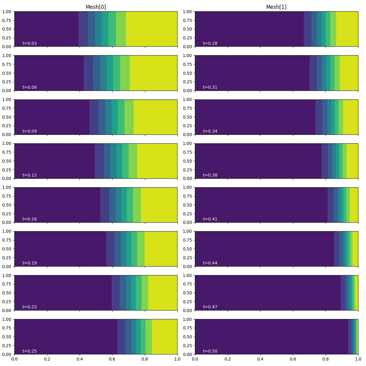
With a time-integrated QoI, the adjoint problem has a source term at the right-hand boundary, rather than a instantaneous pulse at the terminal time. As such, the adjoint solution field accumulates at the right-hand boundary, as well as propagating westwards.

In the next demo, we solve the Burgers problem one last time, but using an object-oriented approach.

This demo can also be accessed as a Python script.