Introduction to mesh movement driven by a Monge-Ampère type equation

In this demo, we consider an example of mesh movement driven by solutions of a Monge-Ampère type equation.

The idea is to consider two domains: the physical domain \(\Omega_P\) and the computational domain \(\Omega_C\). Associated with these are the physical mesh \(\mathcal{H}_P\) and the computational mesh \(\mathcal{H}_C\). The computational domain and mesh remain fixed throughout the simulation, whereas the physical domain and mesh are allowed to change. In this framework, we can interpret mesh movement algorithms as searches for mappings between the computational and physical domains:

\[\mathbf{x}:\Omega_C\rightarrow\Omega_P.\]

In practice we are really searching for a discrete mapping between the computational and physical meshes.

Let \(\boldsymbol{\xi}\) and \(\mathbf{x}\) denote the coordinate fields in the computational and physical domains, respectively. Skipping some of the details that can be found in [MCB18], of the possible mappings we choose one that takes the form

\[\mathbf{x} = \boldsymbol{\xi}+\nabla_{\boldsymbol{\xi}}\phi,\]

where \(\phi\) is a convex potential function. Further, we choose the potential such that it is the solution of the Monge-Ampère type equation,

\[m(\mathbf{x}) \det(\underline{\mathbf{I}}+\nabla_{\boldsymbol{\xi}}\nabla_{\boldsymbol{\xi}}\phi) = \theta,\]

where \(m(\mathbf{x})\) is a so-called monitor function and \(\theta\) is a strictly positive normalisation function. The monitor function is of key importance because it specifies the desired density of the adapted mesh across the domain, i.e., where resolution is focused. Note that density is the reciprocal of area in 2D or of volume in 3D.

We begin the example by importing from the namespaces of Firedrake and Movement.

import os

from firedrake import *

from movement import *

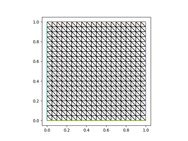
To start with a simple example, consider a uniform mesh of the unit square. Feel free to ignore the “MOVEMENT_REGRESSION_TEST”, as it is only used when this demo is run in the test suite (to reduce its runtime).

test = os.environ.get("MOVEMENT_REGRESSION_TEST")
n = 10 if test else 20
mesh = UnitSquareMesh(n, n)

We can plot the initial mesh using Matplotlib as follows.

import matplotlib.pyplot as plt
from firedrake.pyplot import triplot

fig, axes = plt.subplots()
triplot(mesh, axes=axes)
axes.set_aspect(1)
plt.savefig("monge_ampere1-initial_mesh.jpg")

Let’s choose a monitor function which focuses mesh density in a ring centred within the domain, according to the formula,

\[m(x,y) = 1 + \frac{\alpha}{\cosh^2\left(\beta\left(\left(x-\frac{1}{2}\right)^2+\left(y-\frac{1}{2}\right)^2-\gamma\right)\right)},\]

for some values of the parameters \(\alpha\), \(\beta\), and \(\gamma\). Unity is added at the start to ensure that the monitor function doesn’t get too close to zero.

Here we can think of \(\alpha\) as relating to the amplitude of the monitor function, \(\beta\) as relating to the width of the ring, and \(\gamma\) as the radius of the ring.

def ring_monitor(mesh):
    alpha = Constant(20.0)
    beta = Constant(200.0)
    gamma = Constant(0.15)
    x, y = SpatialCoordinate(mesh)
    r = (x - 0.5) ** 2 + (y - 0.5) ** 2
    return Constant(1.0) + alpha / cosh(beta * (r - gamma)) ** 2

With an initial mesh and a monitor function, we are able to construct a MongeAmpereMover instance and adapt the mesh. By default, the Monge-Ampère equation is solved to a relative tolerance of \(10^{-8}\). However, for the purposes of continuous integration testing, a tolerance of \(10^{-3}\) is used instead to further reduce the runtime.

rtol = 1.0e-03 if test else 1.0e-08
mover = MongeAmpereMover(mesh, ring_monitor, method="quasi_newton", rtol=rtol)
mover.move()

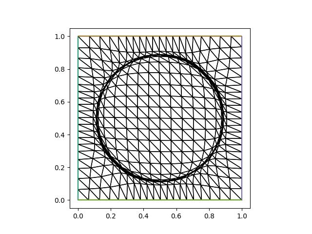
The adapted mesh can be accessed via the mesh attribute of the mover. Plotting it, we see that the adapted mesh has its resolution focused around a ring, as expected.

fig, axes = plt.subplots()
triplot(mover.mesh, axes=axes)
axes.set_aspect(1)
plt.savefig("monge_ampere1-adapted_mesh.jpg")

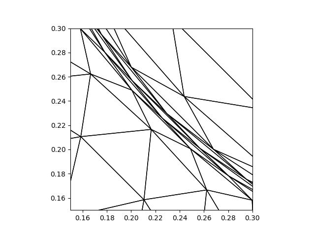
Whilst it looks like the mesh might have tangled elements, closer inspection shows that this is not the case.

fig, axes = plt.subplots()
triplot(mover.mesh, axes=axes)
axes.set_xlim([0.15, 0.3])
axes.set_ylim([0.15, 0.3])
axes.set_aspect(1)
plt.savefig("monge_ampere1-adapted_mesh_zoom.jpg")

Exercise

To further convince yourself that there are no tangled elements, go back to the start of the demo and set up a movement.tangling.MeshTanglingChecker object using the initial mesh. Use it to check for tangling after the mesh movement has been applied.

In the next demo, we will demonstrate that the Monge-Ampère method can also be applied in three dimensions.

This tutorial can be dowloaded as a Python script.

References

[MCB18]

A. T. T. McRae, C. J. Cotter, and J. Budd, C. Optimal-transport-based mesh adaptivity on the plane and sphere using finite elements. SIAM Journal on Scientific Computing, 40(2):1121–1148, 2018. doi:10.1137/16M1109515.