Monge-Ampère mesh movement in three dimensions
In this demo we demonstrate that the Monge-Ampère mesh movement can also be applied to 3D meshes. We employ the sinatan3 function from [] to introduce an interesting pattern.
from firedrake import *
import movement
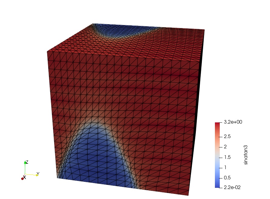
def sinatan3(mesh):
x, y, z = SpatialCoordinate(mesh)
return 0.1 * sin(50 * x * z) + atan2(0.1, sin(5 * y) - 2 * x * z)
We will now try to use mesh movement to optimise the mesh such that it can most accurately represent this function with limited resolution. A good indicator for where resolution is required is to look at the curvature of the function which can be expressed in terms of the norm of the Hessian. A monitor function that targets high resolution in places of high curvature then looks like
where \(:\) indicates the inner product, i.e. \(\sqrt{H:H}\) is the Frobenius norm of \(H\). We have normalised such that the minimum of the monitor function is one (where the error is zero), and its maximum is \(1 + \alpha\) (where the curvature is maximal). This means that we can select the ratio between the largest and smallest cell volume in the moved mesh as \(1+\alpha\).
As in the previous Monge-Ampère demo, we use the
MongeAmpereMover to perform the mesh movement based on
this monitor. We need
to provide the monitor as a callback function that takes the mesh as its
input. During the iterations of the mesh movement process the monitor will then
be re-evaluated in the (iteratively)
moved mesh nodes so that, as we improve the mesh, we can also more accurately
express the monitor function in the desired high-resolution areas.
To track what happens during these iterations, we define a VTK file object
that we will write to in every call when the monitor gets re-evaluated.
from firedrake.output import VTKFile

f = VTKFile("monitor.pvd")
alpha = Constant(10.0)


def monitor(mesh):
    V = FunctionSpace(mesh, "CG", 1)
    # interpolation of the function itself, for output purposes only:
    u = Function(V, name="sinatan3")
    u.interpolate(sinatan3(mesh))

    # NOTE: we are taking the Hessian of the _symbolic_ UFL expression
    # returned by sinatan3(mesh), *not* of the P1 interpolated version
    # stored in u. u is a piecewise linear approximation; Taking its gradient
    # once would result in a piecewise constant (cell-wise) gradient, and taking
    # the gradient of that again would simply be zero.
    hess = grad(grad(sinatan3(mesh)))

    hnorm = Function(V, name="hessian_norm")
    hnorm.interpolate(inner(hess, hess))
    hmax = hnorm.dat.data[:].max()
    f.write(u, hnorm)
    return 1.0 + alpha * hnorm / Constant(hmax)
Let us try this on a fairly coarse unit cube mesh. Note that we use the “relaxation” method (see []), which gives faster convergence for this case.
rtol = 1.0e-08
n = 20
mesh = UnitCubeMesh(n, n, n)
mover = movement.MongeAmpereMover(mesh, monitor, method="relaxation", rtol=rtol)
mover.move()
The results will be written to the monitor.pvd file which represents a series of outputs storing the function and hessian norm evaluated on each of the iteratively moved meshes. This can be viewed, e.g., using ParaView, to produce the following image:
In the next demo, we will demonstrate how to optimise the mesh for the discretisation of a PDE with the aim to minimise its discretisation error.
This tutorial can be dowloaded as a Python script.
References