Using mesh movement to optimise the mesh for PDE solution¶

In this demo we will demonstrate how we might use mesh movement to obtain a mesh that is optimised for solving a particular PDE. The general idea is that we want to reduce numerical error by increasing resolution where the local error is (expected to be) high and decrease it elsewhere.

As an example we will look at the discretisation of the Helmholtz equation

\[ \begin{align}\begin{aligned}-\nabla^2 u + u &= f\\\nabla u \cdot \vec{n} &= 0 \quad \textrm{on}\ \Gamma\end{aligned}\end{align} \]

For an explanation of how we can use Firedrake to implement a Finite Element Method (FEM) discretisation of this PDE see the corresponding Firedrake demo. The only changes we introduce is that we choose a different, slightly more interesting solution \(u\) and rhs \(f\)

\[ \begin{align}\begin{aligned}u(x, y) &= \exp\left(-\frac{(x-x_0)^2 + (y-y_0)^2}{w^2}\right)\\f(x, y) &= -\nabla^2 u(x, y) + u(x, y) = \left[ -\frac{4(x-x_0)^2 + 4(y-y_0)^2}{w^4} + \frac{4}{w^2} + 1 \right] \exp\left(-\frac{(x-x_0)^2 + (y-y_0)^2}{w^2}\right),\end{aligned}\end{align} \]

where \((x_0, y_0)\) is the centre of the Gaussian with width \(w\). Note that here we first choose the solution \(u\) after which we can compute what rhs \(f\) should be, by substitution in the PDE, in order for \(u\) to be the analytical solution. This so-called Method of Manufactured Solutions approach is an easy way to construct PDE configurations for which we know the analytical solution, e.g. for testing purposes.

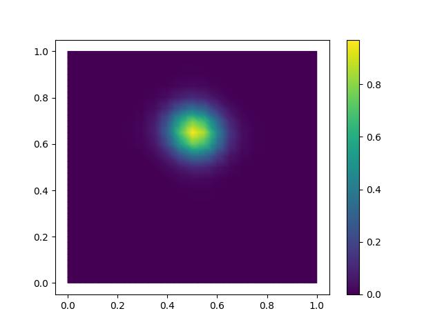
Based on the code in the Firedrake demo, we first solve the PDE on a uniform mesh. Because our chosen solution does not satisfy homogeneous Neumann boundary conditions, we instead apply Dirichlet boundary conditions based on the chosen analytical solution.

import os

from firedrake import *

from movement import MongeAmpereMover

test = os.environ.get("MOVEMENT_REGRESSION_TEST")
n = 10 if test else 20

mesh = UnitSquareMesh(n, n)  # initial mesh


def u_exact(mesh):
    """Return UFL expression of exact solution"""
    x, y = SpatialCoordinate(mesh)
    # some arbitrarily chosen centre (x0, y0) and width w
    w = Constant(0.1)
    x0 = Constant(0.51)
    y0 = Constant(0.65)
    return exp(-((x - x0) ** 2 + (y - y0) ** 2) / w**2)


def solve_helmholtz(mesh):
    """Solve the Helmholtz PDE on the given mesh"""
    V = FunctionSpace(mesh, "CG", 1)
    u = TrialFunction(V)
    v = TestFunction(V)
    u_exact_expr = u_exact(mesh)
    f = -div(grad(u_exact_expr)) + u_exact_expr
    a = (inner(grad(u), grad(v)) + inner(u, v)) * dx
    L = inner(f, v) * dx
    u = Function(V)
    bcs = DirichletBC(V, u_exact_expr, "on_boundary")
    solve(a == L, u, bcs=bcs)
    return u


u_h = solve_helmholtz(mesh)

import matplotlib.pyplot as plt
from firedrake.pyplot import tripcolor

fig, axes = plt.subplots()
contours = tripcolor(u_h, axes=axes)
fig.colorbar(contours)
plt.savefig("monge_ampere_helmholtz-initial_solution.jpg")

../_images/monge_ampere_helmholtz-initial_solution.jpg

As in the Helmholtz demo, we can compute the L2-norm of the numerical error:

error = u_h - u_exact(mesh)
print("L2-norm error on initial mesh:", sqrt(assemble(dot(error, error) * dx)))

L2-norm error on initial mesh: 0.010233816824277465

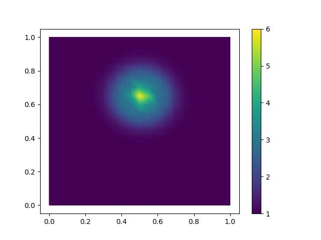
We will now try to use mesh movement to optimise the mesh to reduce this numerical error. We use the same monitor function as in the previous Monge-Ampère demo based on the norm of the Hessian of the solution. In the following implementation we use the exact solution \(u_{\text{exact}}\) which we have as a symbolic UFL expression, and thus we can also obtain the Hessian symbolically as grad(grad(u_exact)). To compute its maximum norm however we do interpolate it to a P1 function space V and take the maximum of the array of nodal values.

alpha = Constant(5.0)


def monitor(mesh):
    V = FunctionSpace(mesh, "CG", 1)
    Hnorm = Function(V, name="Hnorm")
    H = grad(grad(u_exact(mesh)))
    Hnorm.interpolate(sqrt(inner(H, H)))
    Hnorm_max = Hnorm.dat.data.max()
    m = 1 + alpha * Hnorm / Hnorm_max
    return m

Plot the monitor function on the original mesh

fig, axes = plt.subplots()
m = Function(u_h, name="monitor")
m.interpolate(monitor(mesh))
contours = tripcolor(m, axes=axes)
fig.colorbar(contours)
plt.savefig("monge_ampere_helmholtz-monitor.jpg")
fig, axes = plt.subplots()

../_images/monge_ampere_helmholtz-monitor.jpg

rtol = 1.0e-03 if test else 1.0e-08
mover = MongeAmpereMover(mesh, monitor, method="quasi_newton", rtol=rtol)
mover.move()

For every iteration the MongeAmpereMover prints the minimum to maximum ratio of the cell areas in the mesh, the residual in the Monge Ampere equation, and the coefficient of variation of the cell areas:

 Min/Max 2.0268e-01   Residual 4.7659e-01   Variation (σ/μ) 9.9384e-01
 Min/Max 3.7852e-01   Residual 2.4133e-01   Variation (σ/μ) 9.9659e-01
 Min/Max 5.9791e-01   Residual 1.2442e-01   Variation (σ/μ) 9.9774e-01
 Min/Max 7.1000e-01   Residual 6.5811e-02   Variation (σ/μ) 9.9804e-01
 Min/Max 7.7704e-01   Residual 3.4929e-02   Variation (σ/μ) 9.9818e-01
 Min/Max 8.3434e-01   Residual 1.7261e-02   Variation (σ/μ) 9.9829e-01
 Min/Max 8.5805e-01   Residual 7.7528e-03   Variation (σ/μ) 9.9833e-01
 Min/Max 8.6653e-01   Residual 3.1551e-03   Variation (σ/μ) 9.9835e-01
 Min/Max 8.6796e-01   Residual 1.1644e-03   Variation (σ/μ) 9.9835e-01
 Min/Max 8.6792e-01   Residual 3.8816e-04   Variation (σ/μ) 9.9835e-01
 Min/Max 8.6784e-01   Residual 1.1574e-04   Variation (σ/μ) 9.9835e-01
 Min/Max 8.6778e-01   Residual 1.5645e-05   Variation (σ/μ) 9.9835e-01
 Min/Max 8.6776e-01   Residual 7.5654e-06   Variation (σ/μ) 9.9835e-01
 Min/Max 8.6776e-01   Residual 3.5803e-06   Variation (σ/μ) 9.9835e-01
 Min/Max 8.6775e-01   Residual 1.5113e-06   Variation (σ/μ) 9.9835e-01
 Min/Max 8.6775e-01   Residual 5.7080e-07   Variation (σ/μ) 9.9835e-01
 Min/Max 8.6775e-01   Residual 1.9357e-07   Variation (σ/μ) 9.9835e-01
 Min/Max 8.6775e-01   Residual 5.8585e-08   Variation (σ/μ) 9.9835e-01
Converged in 17 iterations.

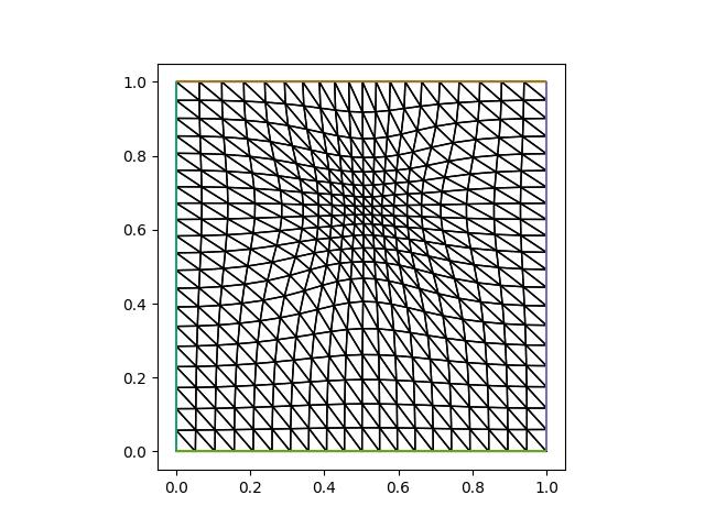
Plotting the resulting mesh:

from firedrake.pyplot import triplot

fig, axes = plt.subplots()
triplot(mover.mesh, axes=axes)
axes.set_aspect(1)
plt.savefig("monge_ampere_helmholtz-adapted_mesh.jpg")

../_images/monge_ampere_helmholtz-adapted_mesh.jpg

Now let us see whether the numerical error has actually been reduced if we solve the PDE on this mesh:

u_h = solve_helmholtz(mover.mesh)
error = u_h - u_exact(mover.mesh)
print("L2-norm error on moved mesh:", sqrt(assemble(dot(error, error) * dx)))

L2-norm error on moved mesh: 0.005955820168534556

Of course, in many practical problems we do not actually have access to the exact solution. We can then use the Hessian of the numerical solution in the monitor function. When calculating the Hessian we have to be a bit careful however: since our numerical FEM solution \(u_h\) is a piecewise linear function, its first gradient results in a piecewise constant function, a vector-valued constant function in each cell. Taking its gradient in each cell would therefore simply be zero. Instead, we should numerically approximate the derivatives to “recover” the Hessian, for which there are a number of different methods.

As Hessians are often used in metric-based h-adaptivity, some of these methods have been implemented in the animate package. An implementation of a monitor based on the Hessian of the numerical solution is given below. Note that this requires solving the Helmholtz PDE in every mesh movement iteration, and thus may become significantly slower for large problems.

from animate import RiemannianMetric


def monitor2(mesh):
    u_h = solve_helmholtz(mesh)
    V = FunctionSpace(mesh, "CG", 1)
    TV = TensorFunctionSpace(mesh, "CG", 1)
    H = RiemannianMetric(TV)
    H.compute_hessian(u_h, method="L2")

    Hnorm = Function(V, name="Hnorm")
    Hnorm.interpolate(sqrt(inner(H, H)))
    Hnorm_max = Hnorm.dat.data.max()
    m = 1 + alpha * Hnorm / Hnorm_max
    return m


mover = MongeAmpereMover(mesh, monitor2, method="quasi_newton", rtol=rtol)
mover.move()

u_h = solve_helmholtz(mover.mesh)
error = u_h - u_exact(mover.mesh)
print("L2-norm error on moved mesh:", sqrt(assemble(dot(error, error) * dx)))

L2-norm error on moved mesh: 0.00630874419681285

This tutorial can be dowloaded as a Python script.