Solving ordinary differential equations using Goalie
Goalie was designed primarily with partial differential equations (PDEs) in mind. However, it can also be used to solve ordinary differential equations (ODEs).
For example, consider the scalar, linear ODE,
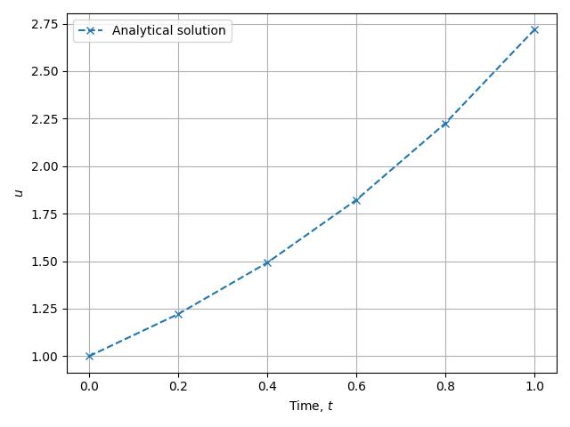
which we solve for \(u(t)\) over the time period \(t\in(0,1]\). It is straightforward to verify that this ODE has analytical solution
Given a sample of points in time, we can plot this as follows.
import matplotlib.pyplot as plt
import numpy as np

dt = 0.2
times = np.arange(0, 1.01, dt)

fig, axes = plt.subplots()
axes.plot(times, np.exp(times), "--x", label="Analytical solution")
axes.set_xlabel(r"Time, $t$")
axes.set_ylabel(r"$u$")
axes.grid(True)
axes.legend()
plt.tight_layout()
plt.savefig("ode-analytical.jpg")
In this demo, we solve the above ODE numerically using three different timestepping schemes and compare the results.
First, import from the namespaces of Firedrake and Goalie.
from firedrake import *

from goalie import *
Next, create a simple TimeInterval object to hold information related to
the time discretisation. This is a simplified version of TimePartition,
which only has one subinterval.
end_time = 1
time_partition = TimeInterval(end_time, dt, "u")
Much of the following might seem excessive for this example. However, it exists to allow for the flexibility required in later PDE examples.
We need to create a FunctionSpace for the solution field to live in. Given
that we have a scalar ODE, the solution is just a real number at each time level. We
represent this using the degree-0 \(R\)-space, as follows. A mesh is required to
define a function space in Firedrake, although what the mesh is doesn’t actually
matter for this example.
def get_function_spaces(mesh):
    return {"u": FunctionSpace(mesh, "R", 0)}
Next, we need to supply the initial condition \(u(0) = 1\). We do this by creating
a Function in the \(R\)-space and assigning it the value 1.
def get_initial_condition(point_seq):
    fs = point_seq.function_spaces["u"][0]
    return {"u": Function(fs).assign(1.0)}
The first timestepping scheme we consider is Forward Euler, which is also known as Explicit Euler because it approximates the solution at time level \(i+1\) as an explicit function of solution approximation at time level \(i\).
where \(u_k\) denotes the approximation at time level k and \(\Delta k\) is the timestep length. This expression may be rearranged as
Even though there are no spatial derivatives in our problem, we still have to represent the problem in a finite element formulation in order to solve it using Goalie. Recall that functions in our function space, \(R\) are just scalar valued. To use the finite element notation, we multiply both sides of the equation by a test function and integrate:
It’s worth noting that integration over an \(R\)-space amounts to summation and because we have a scalar \(R\)-space it is a summation of a single value. Again, this machinery may seem excessive but it becomes necessary for PDE problems.
The Forward Euler scheme may be implemented as follows.
def get_form_forward_euler(point_seq):
    def form(index):
        R = point_seq.function_spaces["u"][index]
        v = TestFunction(R)
        u, u_ = point_seq.fields["u"]
        dt = Function(R).assign(point_seq.time_partition.timesteps[index])

        # Setup variational problem
        F = (u - u_ - dt * u_) * v * dx
        return {"u": F}

    return form
We have a method defining the Forward Euler scheme. To put it into practice, we need to define the solver. This boils down to applying the update repeatedly in a time loop.
def get_solver(point_seq):
    def solver(index):
        tp = point_seq.time_partition

        # Get the current and lagged solutions
        u, u_ = point_seq.fields["u"]

        # Define the (trivial) form
        F = point_seq.form(index)["u"]

        # Since the form is trivial, we can solve with a single application of a Jacobi
        # preconditioner
        sp = {"ksp_type": "preonly", "pc_type": "jacobi"}

        # Time integrate from t_start to t_end
        dt = tp.timesteps[index]
        t_start, t_end = tp.subintervals[index]
        t = t_start
        while t < t_end - 1.0e-05:
            solve(F == 0, u, solver_parameters=sp)
            yield

            u_.assign(u)
            t += dt

    return solver
For this ODE problem, the main driver object is a PointSeq, which is
defined in terms of the TimePartition describing the time discretisation,
plus the functions defined above.
point_seq = PointSeq(
    time_partition,
    get_function_spaces=get_function_spaces,
    get_initial_condition=get_initial_condition,
    get_form=get_form_forward_euler,
    get_solver=get_solver,
)
We can solve the ODE using the solve_forward() method and extract the
solution trajectory as follows. The method returns a nested dictionary of solutions,
with the first key specifying the field name and the second key specifying the type of
solution field. For the purposes of this demo, we have field "u", which is a
forward solution. The resulting solution trajectory is a list.
solutions = point_seq.solve_forward()["u"]["forward"]
Note that the solution trajectory does not include the initial value, so we prepend it.
We also convert the solution Functions to floats, for plotting
purposes. Whilst there is only one subinterval in this example, we show how to loop
over subintervals, as this is instructive for the general case.
forward_euler_trajectory = [1]
forward_euler_trajectory += [
    float(sol) for subinterval in solutions for sol in subinterval
]
Plot the trajectory and compare it against the analytical solution.
fig, axes = plt.subplots()
axes.plot(times, np.exp(times), "--x", label="Analytical solution")
axes.plot(times, forward_euler_trajectory, "--+", label="Forward Euler")
axes.set_xlabel(r"Time, $t$")
axes.set_ylabel(r"$u$")
axes.grid(True)
axes.legend()
plt.tight_layout()
plt.savefig("ode-forward_euler.jpg")
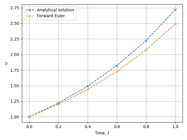
The Forward Euler approximation to the analytical solution isn’t terrible, but clearly consistently underestimates. Now let’s try using Backward Euler, also known as Implicit Euler because the approximation at the next time level is represented as an implicit function of the approximation at the current time level:
Similarly to the above, this gives rise to
def get_form_backward_euler(point_seq):
    def form(index):
        R = point_seq.function_spaces["u"][index]
        v = TestFunction(R)
        u, u_ = point_seq.fields["u"]
        dt = Function(R).assign(point_seq.time_partition.timesteps[index])

        # Setup variational problem
        F = (u - u_ - u * dt) * v * dx
        return {"u": F}

    return form
To apply Backward Euler we create the PointSeq in the same way, just with
get_form_forward_euler substituted for get_form_backward_euler.
point_seq = PointSeq(
    time_partition,
    get_function_spaces=get_function_spaces,
    get_initial_condition=get_initial_condition,
    get_form=get_form_backward_euler,
    get_solver=get_solver,
)
solutions = point_seq.solve_forward()["u"]["forward"]

backward_euler_trajectory = [1]
backward_euler_trajectory += [
    float(sol) for subinterval in solutions for sol in subinterval
]

fig, axes = plt.subplots()
axes.plot(times, np.exp(times), "--x", label="Analytical solution")
axes.plot(times, forward_euler_trajectory, "--+", label="Forward Euler")
axes.plot(times, backward_euler_trajectory, "--o", label="Backward Euler")
axes.set_xlabel(r"Time, $t$")
axes.set_ylabel(r"$u$")
axes.grid(True)
axes.legend()
plt.tight_layout()
plt.savefig("ode-backward_euler.jpg")
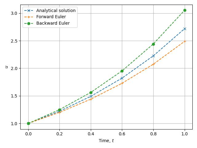
This time we see that Implicit Euler consistenly overestimates the solution. Both of the methods we’ve considered so far are first order methods. To get a better result, we combine them to obtain the second order Crank-Nicolson method:
where \(\theta\in(0,1)\). The standard choice is to take \(\theta=\frac12\).
def get_form_crank_nicolson(point_seq):
    def form(index):
        R = point_seq.function_spaces["u"][index]
        v = TestFunction(R)
        u, u_ = point_seq.fields["u"]
        dt = Function(R).assign(point_seq.time_partition.timesteps[index])
        theta = Function(R).assign(0.5)

        # Setup variational problem
        F = (u - u_ - dt * (theta * u + (1 - theta) * u_)) * v * dx
        return {"u": F}

    return form


point_seq = PointSeq(
    time_partition,
    get_function_spaces=get_function_spaces,
    get_initial_condition=get_initial_condition,
    get_form=get_form_crank_nicolson,
    get_solver=get_solver,
)

solutions = point_seq.solve_forward()["u"]["forward"]
crank_nicolson_trajectory = [1]
crank_nicolson_trajectory += [
    float(sol) for subinterval in solutions for sol in subinterval
]

fig, axes = plt.subplots()
axes.plot(times, np.exp(times), "--x", label="Analytical solution")
axes.plot(times, forward_euler_trajectory, "--+", label="Forward Euler")
axes.plot(times, backward_euler_trajectory, "--o", label="Backward Euler")
axes.plot(times, crank_nicolson_trajectory, "--*", label="Crank-Nicolson")
axes.set_xlabel(r"Time, $t$")
axes.set_ylabel(r"$u$")
axes.grid(True)
axes.legend()
plt.tight_layout()
plt.savefig("ode-crank_nicolson.jpg")
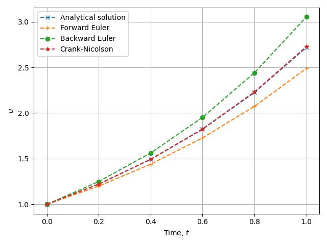
With this method, we see that the approximation is of much higher quality. Another way to see this is to compare the approximations of \(e\) given by each approach:
print(f"e to 9 d.p.:    {np.exp(1):.9f}")
print(f"Forward Euler:  {forward_euler_trajectory[-1]:.9f}")
print(f"Backward Euler: {backward_euler_trajectory[-1]:.9f}")
print(f"Crank-Nicolson: {crank_nicolson_trajectory[-1]:.9f}")
e to 9 d.p.:    2.718281828
Forward Euler:  2.488320000
Backward Euler: 3.051757812
Crank-Nicolson: 2.727412827
In the next demo, we move on to solve a partial differential
equation (PDE) using a MeshSeq.
This demo can also be accessed as a Python script.