Burgers equation with Goal-oriented mesh adaptation
In the Hessian-based adaptation, we applied a Hessian-based mesh adaptation to the time-dependent Burgers equation. Here, we alternatively consider a goal-oriented error estimation to drive the mesh adaptation. Again, we will choose to partition the problem over multiple subintervals and hence multiple meshes to adapt. We also chose to apply a QoI which integrates in time as well as space.
We copy over the setup as before.
import matplotlib.pyplot as plt
from animate.adapt import adapt
from animate.metric import RiemannianMetric
from firedrake import *

from goalie import *

n = 32
meshes = [UnitSquareMesh(n, n), UnitSquareMesh(n, n)]
fields = [Field("u", family="Lagrange", degree=2, vector=True)]


def get_initial_condition(mesh_seq):
    fs = mesh_seq.function_spaces["u"][0]
    x, y = SpatialCoordinate(mesh_seq[0])
    return {"u": Function(fs).interpolate(as_vector([sin(pi * x), 0]))}
The solver and QoI are as described in the Burgers with a time-integrated QoI demo.
def get_solver(mesh_seq):
    def solver(index):
        u, u_ = mesh_seq.field_functions["u"]

        # Define constants
        R = FunctionSpace(mesh_seq[index], "R", 0)
        dt = Function(R).assign(mesh_seq.time_partition.timesteps[index])
        nu = Function(R).assign(0.0001)

        # Setup variational problem
        v = TestFunction(u.function_space())
        F = (
            inner((u - u_) / dt, v) * dx
            + inner(dot(u, nabla_grad(u)), v) * dx
            + nu * inner(grad(u), grad(v)) * dx
        )

        # Communicate variational form to mesh_seq
        mesh_seq.read_forms({"u": F})

        # Time integrate from t_start to t_end
        tp = mesh_seq.time_partition
        t_start, t_end = tp.subintervals[index]
        dt = tp.timesteps[index]
        t = t_start
        qoi = mesh_seq.get_qoi(index)
        while t < t_end - 1.0e-05:
            solve(F == 0, u, ad_block_tag="u")
            mesh_seq.J += qoi(t)
            yield

            u_.assign(u)
            t += dt

    return solver


def get_qoi(mesh_seq, i):
    R = FunctionSpace(mesh_seq[i], "R", 0)
    dt = Function(R).assign(mesh_seq.time_partition.timesteps[i])

    def time_integrated_qoi(t):
        u = mesh_seq.field_functions["u"][0]
        return dt * inner(u, u) * ds(2)

    return time_integrated_qoi
We use the mesh setup and time partitioning involving two meshes, as in a previous demo, except that we export every timestep rather than every other timestep.
end_time = 0.5
dt = 1 / n
num_subintervals = len(meshes)
time_partition = TimePartition(
    end_time,
    num_subintervals,
    dt,
    fields,
    num_timesteps_per_export=1,
)
Since we want to do goal-oriented mesh adaptation, we use a
GoalOrientedMeshSeq.
mesh_seq = GoalOrientedMeshSeq(
    time_partition,
    meshes,
    get_initial_condition=get_initial_condition,
    get_solver=get_solver,
    get_qoi=get_qoi,
    qoi_type="time_integrated",
)
Compared to the previous Hessian-based adaptation,
this adaptor depends on adjoint solution data as well as forward solution data.
For simplicity, we begin by using
compute_isotropic_metric().
def adaptor(mesh_seq, solutions=None, indicators=None):
    metrics = []
    complexities = []

    indicators = mesh_seq.indicators

    # Ramp the target average metric complexity per fixed point iteration
    base, target, iteration = 400, 1000, mesh_seq.fp_iteration
    mp = {
        "dm_plex_metric": {
            "target_complexity": ramp_complexity(base, target, iteration),
            "p": 1.0,
            "h_min": 1.0e-04,
            "h_max": 2,
        }
    }

    # Construct the metric on each subinterval
    for i, mesh in enumerate(mesh_seq):
        dt = mesh_seq.time_partition.timesteps[i]

        P1_ten = TensorFunctionSpace(mesh, "CG", 1)
        metrics_subinterval = []

        # Calculate metric at each timestep
        for indi in indicators["u"][i]:
            # timestep instance of Riemanian metric
            metric_timestep = RiemannianMetric(P1_ten)
            metric_timestep.set_parameters(mp)

            # Deduce an isotropic metric from the error indicator field
            metric_timestep.compute_isotropic_metric(
                error_indicator=indi, interpolant="L2"
            )
            metric_timestep.normalise()

            # Append the metric for the step in the time partition
            metrics_subinterval.append(metric_timestep)

        # Set the first metric as the base and average remaining
        metrics_subinterval[0].average(
            *metrics_subinterval[1:], weights=[dt] * len(metrics_subinterval)
        )

        metrics.append(metrics_subinterval[0])

    # Apply space time normalisation
    space_time_normalise(metrics, mesh_seq.time_partition, mp)

    # Adapt each mesh w.r.t. the corresponding metric, provided it hasn't converged
    for i, metric in enumerate(metrics):
        if not mesh_seq.converged[i]:
            mesh_seq[i] = adapt(mesh_seq[i], metric)
        complexities.append(metric.complexity())
    num_dofs = mesh_seq.count_vertices()
    num_elem = mesh_seq.count_elements()
    pyrint(f"fixed point iteration {iteration + 1}:")
    for i, (complexity, ndofs, nelem) in enumerate(
        zip(complexities, num_dofs, num_elem, strict=True)
    ):
        pyrint(
            f"  subinterval {i}, complexity: {complexity:4.0f}"
            f", dofs: {ndofs:4d}, elements: {nelem:4d}"
        )

    # Plot each intermediate adapted mesh
    fig, axes = mesh_seq.plot()
    for i, ax in enumerate(axes):
        ax.set_title(f"Subinterval {i + 1}")
    fig.savefig(f"burgers-isotropic_mesh{iteration + 1}.jpg")
    plt.close()

    # Since we have two subintervals, we should check if the target complexity has been
    # (approximately) reached on each subinterval
    continue_unconditionally = np.array(complexities) < 0.90 * target
    return continue_unconditionally
With the adaptor function defined, we can call the fixed point iteration method.
params = GoalOrientedAdaptParameters(
    {
        "element_rtol": 0.001,
        "maxiter": 35,
    }
)

solutions = mesh_seq.fixed_point_iteration(
    adaptor,
    enrichment_kwargs={"enrichment_method": "h"},
    parameters=params,
)
This time, we find that the fixed point iteration converges in four iterations. Convergence is reached because the relative change in QoI is found to be smaller than the default tolerance.
fixed point iteration 1:
  subinterval 0, complexity:  448, dofs:  608, elements: 1140
  subinterval 1, complexity:  351, dofs:  463, elements:  854
fixed point iteration 2:
  subinterval 0, complexity:  654, dofs:  772, elements: 1442
  subinterval 1, complexity:  539, dofs:  649, elements: 1207
fixed point iteration 3:
  subinterval 0, complexity:  883, dofs:  988, elements: 1869
  subinterval 1, complexity:  710, dofs:  809, elements: 1509
QoI converged after 4 iterations under relative tolerance 0.001.
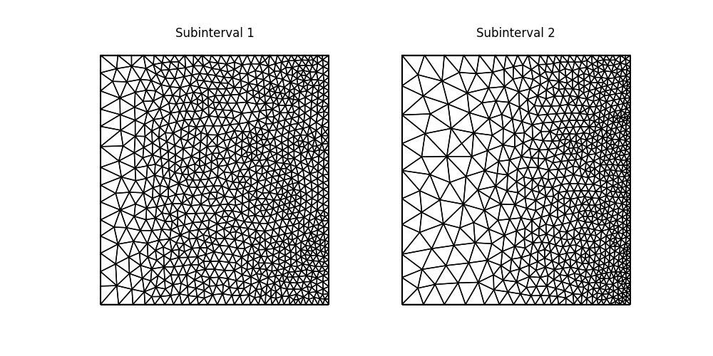
Let’s plot the final converged and adapted meshes.
fig, axes = mesh_seq.plot()
for i, ax in enumerate(axes):
    ax.set_title(f"Subinterval {i + 1}")
fig.savefig("burgers-isotropic_mesh.jpg")
plt.close()

Looking at the final adapted mesh, we can make a few observations. Firstly, the mesh elements are indeed isotropic. Secondly, the solution moves to the right, becoming more densely distributed near to the right-hand boundary. This can be seen by comparing the second mesh against the first.
Recall that the Burgers problem is quasi-1D, since the analytical solution varies in the \(x\)-direction, but is constant in the \(y\)-direction, suggesting a more optimal choice of goal-based error estimation for this problem is one which accounts for this anisotopy.
Goalie also provide support for anisotropic goal-oriented mesh adaptation. Here,
we consider the compute_anisotropic_dwr_metric() driver.
(See documentation for details.) To use it, we just need to define
a different adaptor function. The same error indicator is used as
for the isotropic approach. Additionally, the Hessian of the forward
solution is estimated as in the
Hessian-based adaptation
to give anisotropy to the metric.
For this driver, normalisation is handled differently than for
compute_isotropic_metric(), where the
normalise() method is called after
construction. In this case, the metric is already normalised within
the call to compute_anisotropic_dwr_metric(),
so this is not required.
def adaptor(mesh_seq, solutions=None, indicators=None):
    metrics = []
    complexities = []

    solutions = mesh_seq.solutions
    indicators = mesh_seq.indicators

    # Ramp the target average metric complexity per timestep
    base, target, iteration = 400, 1000, mesh_seq.fp_iteration
    mp = {
        "dm_plex_metric": {
            "target_complexity": ramp_complexity(base, target, iteration),
            "p": 1.0,
            "h_min": 1.0e-04,
            "h_max": 2,
        }
    }

    # Construct the metric on each subinterval
    for i, mesh in enumerate(mesh_seq):
        sols = solutions["u"]["forward"][i]
        dt = mesh_seq.time_partition.timesteps[i]
        P1_ten = TensorFunctionSpace(mesh, "CG", 1)
        metrics_subinterval = []

        # Calculate metric at each timestep
        for j, sol in enumerate(sols):
            # get indicator
            indi = indicators["u"][i][j]
            # timestep instance of Riemanian metric
            metric_timestep = RiemannianMetric(P1_ten)

            # At each timestep, recover Hessians of the two components of the solution
            # vector combine with metric intersection.
            hessians = [RiemannianMetric(P1_ten) for _ in range(2)]
            for k, hessian in enumerate(hessians):
                hessian.set_parameters(mp)
                hessian.compute_hessian(sol[k])
                hessian.enforce_spd(restrict_sizes=True)
            hessians[0].intersect(hessians[1])
            metric_timestep.set_parameters(mp)

            # Deduce an anisotropic metric from the error indicator field
            metric_timestep.compute_anisotropic_dwr_metric(
                indi, hessians[0], interpolant="L2"
            )

            # Append the metric for the step in the time partition
            metrics_subinterval.append(metric_timestep)

        # Set the first metric as the base and average remaining
        metrics_subinterval[0].average(
            *metrics_subinterval[1:], weights=[dt] * len(metrics_subinterval)
        )

        metrics.append(metrics_subinterval[0])

    # Apply space time normalisation
    space_time_normalise(metrics, mesh_seq.time_partition, mp)

    # Adapt each mesh w.r.t. the corresponding metric, provided it hasn't converged
    for i, metric in enumerate(metrics):
        if not mesh_seq.converged[i]:
            mesh_seq[i] = adapt(mesh_seq[i], metric)
        complexities.append(metric.complexity())
    num_dofs = mesh_seq.count_vertices()
    num_elem = mesh_seq.count_elements()
    pyrint(f"fixed point iteration {iteration + 1}:")
    for i, (complexity, ndofs, nelem) in enumerate(
        zip(complexities, num_dofs, num_elem, strict=False)
    ):
        pyrint(
            f"  subinterval {i}, complexity: {complexity:4.0f}"
            f", dofs: {ndofs:4d}, elements: {nelem:4d}"
        )

    # Plot each intermediate adapted mesh
    fig, axes = mesh_seq.plot()
    for i, ax in enumerate(axes):
        ax.set_title(f"Subinterval {i + 1}")
    fig.savefig(f"burgers-anisotropic_mesh{iteration + 1}.jpg")
    plt.close()

    # Since we have multiple subintervals, we should check if the target complexity has
    # been (approximately) reached on each subinterval
    continue_unconditionally = np.array(complexities) < 0.90 * target
    return continue_unconditionally
To avoid confusion, we redefine the GoalOrientedMeshSeq object before using
it.
mesh_seq = GoalOrientedMeshSeq(
    time_partition,
    meshes,
    get_initial_condition=get_initial_condition,
    get_solver=get_solver,
    get_qoi=get_qoi,
    qoi_type="time_integrated",
)

solutions = mesh_seq.fixed_point_iteration(
    adaptor,
    enrichment_kwargs={"enrichment_method": "h"},
    parameters=params,
)
We find that the fixed point iteration again converges in four iterations.
fixed point iteration 1:
  subinterval 0, complexity:  460, dofs:  596, elements: 1084
  subinterval 1, complexity:  337, dofs:  428, elements:  781
fixed point iteration 2:
  subinterval 0, complexity:  687, dofs:  837, elements: 1547
  subinterval 1, complexity:  506, dofs:  608, elements: 1122
fixed point iteration 3:
  subinterval 0, complexity:  907, dofs:  1062, elements: 1979
  subinterval 1, complexity:  682, dofs:  800,  elements: 1490
QoI converged after 4 iterations under relative tolerance 0.001.
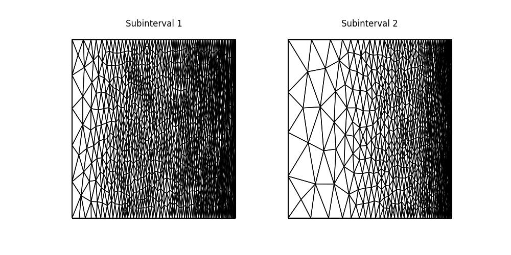
Finally, let’s plot the final converged and adapted meshes.
fig, axes = mesh_seq.plot()
for i, ax in enumerate(axes):
    ax.set_title(f"Subinterval {i + 1}")
fig.savefig("burgers-anisotropic_mesh.jpg")
plt.close()

The mesh is similar to the isotropic case but more anisotropic, based on information from the Hessian of the adjoint solution. In this anisotropic mesh there is a larger size and shape range between smaller elements on the right, concentrated where the solution is moving and larger elements on the left, where there is little contribution to the overall QoI.
This demo can also be accessed as a Python script.