Mesh movement using the lineal spring approach

In this demo, we demonstrate a basic example using the lineal spring method, as described in [Farhat et al., 1998]. For simplicity of presentation, we consider a very similar example to that considered in the Laplacian smoothing demo, where mesh movement is driven by enforcing a particular displacement of the top boundary of a square mesh.

The idea of the lineal spring method is to re-interpret the edges of a mesh as a structure of stiff beams. Each beam has a stiffness associated with it, which is related to its length and its orientation. We can assemble this information as a stiffness matrix,

$$\begin{array}{r}\underset{―}{\mathbf{K}}=\left[\begin{array}{ccccc}\underset{―}{{\mathbf{K}}_{11}}& & \dots & & \underset{―}{{\mathbf{K}}_{1N}}\\ ⋮& & \ddots & & ⋮\\ \underset{―}{{\mathbf{K}}_{N1}}& & \dots & & \underset{―}{{\mathbf{K}}_{NN}}\end{array}\right],\end{array}$$

where $N$ is the number of vertices in the mesh and each block $\underset{―}{{\mathbf{K}}_{ij}}$ is a zero matrix if and only if vertex $i$ is not connected to vertex $j$. For a 2D problem, each $\underset{―}{{\mathbf{K}}_{ij}}\in {\mathbb{R}}^{2\times 2}$ and $\underset{―}{\mathbf{K}}\in {\mathbb{R}}^{2N\times 2N}$.

As with the Laplacian smoothing method, the lineal spring approach relies on there being a user-specified boundary condition, but note that it is now expressed as a boundary displacement, rather than a boundary velocity. Then we are able to compute the displacement of the vertices by solving the linear system

$$\underset{―}{\mathbf{K}}\mathbf{u}=\mathbf{0},$$

where $\mathbf{u}\in {\mathbb{R}}^{2N}$ is a ‘flattened’ version of the displacement vector. By solving this equation, we see how the structure of beams responds to the forced boundary displacement.

There are two main differences to note with the Laplacian smoothing approach. The first is that Laplacian smoothing is formulated in terms of mesh velocity, whereas this method is formulated in terms of displacements. Secondly, the mesh velocity $\mathbf{v}$ in the Laplacian smoothing method may be approximated at timestep $n$ as

$${\mathbf{v}}_n\approx \frac{{\mathbf{x}}_n-{\mathbf{x}}_{n-1}}{\mathrm{\Delta }t},$$

where ${\mathbf{x}}_n$ are the mesh coordinates at timestep $n$ and $\mathrm{\Delta }t$ is the timestep length. In the lineal spring method, however, we solve for the overall displacement, which at timestep $n$ takes the form

$${\mathbf{u}}_n={\mathbf{x}}_n-{\mathbf{x}}_0.$$

So Laplacian smoothing is related to recent changes in velocity, whereas the lineal spring method considered here is concerned with changes in position since the start of the simulation.

We begin by importing from the namespaces of Firedrake and Movement.

import matplotlib.pyplot as plt
from firedrake import *
from firedrake.pyplot import triplot

from movement import *

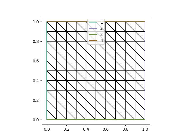
Recall the initial uniform mesh of the unit square used in the Laplacian smoothing demo, which has four boundary segments tagged with the integers 1, 2, 3, and 4. Note that segment 4 corresponds to the top boundary.

n = 10
mesh = UnitSquareMesh(n, n)
coord_data_init = mesh.coordinates.dat.data.copy()
fig, axes = plt.subplots()
triplot(mesh, axes=axes)
axes.set_aspect(1)
axes.legend()
plt.savefig("lineal_spring-initial_mesh.jpg")

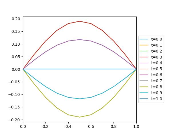
We consider the same time-dependent forcing to the top boundary and see how the mesh structure responds. We use a very similar formula,

$${\mathbf{u}}_f(x,y,t)=[0,A\sin \left(\frac{2\pi t}{T}\right)\sin (\pi x)],$$

where $A$ is the amplitude and $T$ is the time period, but again note that it is now expressed as a boundary displacement ${\mathbf{u}}_f$:, rather than a boundary velocity. As such, we should not expect the boundary movement to be the same.

import numpy as np

bd_period = 1.0
num_timesteps = 10
timestep = bd_period / num_timesteps
bd_amplitude = 0.2


def boundary_displacement(x, t):
    return bd_amplitude * np.sin(2 * pi * t / bd_period) * np.sin(pi * x)


X = np.linspace(0, 1, n + 1)
times = np.arange(0, bd_period + 0.5 * timestep, timestep)

fig, axes = plt.subplots()
for time in times:
    axes.plot(X, boundary_displacement(X, time), label=f"t={time:.1f}")
axes.set_xlim([0, 1])
axes.legend()
box = axes.get_position()
axes.set_position([box.x0, box.y0, box.width * 0.8, box.height])
axes.legend(loc="center left", bbox_to_anchor=(1, 0.5))
plt.savefig("lineal_spring-boundary_displacement.jpg")

To apply this boundary displacement, we need to create a SpringMover instance and define a function for updating the boundary conditions.

mover = SpringMover(mesh, timestep, method="lineal")
top = Function(mover.coord_space)
moving_boundary = DirichletBC(mover.coord_space, top, 4)


def update_boundary_displacement(t):
    coord_data = mover.mesh.coordinates.dat.data
    bd_data = top.dat.data
    for i in moving_boundary.nodes:
        x, y = coord_data[i]
        bd_data[i][1] = boundary_displacement(x, t)

In addition to the moving boundary, we specify the remaining boundaries to be fixed.

fixed_boundaries = DirichletBC(mover.coord_space, 0, [1, 2, 3])
boundary_conditions = (fixed_boundaries, moving_boundary)

We are now able to apply the mesh movement method.

import matplotlib.patches as mpatches

fig, axes = plt.subplots(ncols=4, nrows=3, figsize=(12, 10))
for i, time in enumerate(times):
    idx = 0 if i == 0 else i + 1

    # Move the mesh and calculate the displacement
    mover.move(
        time,
        update_boundary_displacement=update_boundary_displacement,
        boundary_conditions=boundary_conditions,
    )

    # Plot the current mesh, adding a time label
    ax = axes[idx // 4, idx % 4]
    triplot(mover.mesh, axes=ax)
    ax.legend(handles=[mpatches.Patch(label=f"t={time:.1f}")], handlelength=0)
    ax.set_ylim([-0.05, 1.45])
axes[0, 1].axis(False)
plt.savefig("lineal_spring-adapted_meshes.jpg")

This should give command line output similar to the following:

0.00   Volume ratio  1.00   Variation (σ/μ) 5.16e-16   Displacement 0.00 m
0.10   Volume ratio  1.02   Variation (σ/μ) 4.23e-03   Displacement 0.05 m
0.20   Volume ratio  1.05   Variation (σ/μ) 1.11e-02   Displacement 0.08 m
0.30   Volume ratio  1.09   Variation (σ/μ) 1.82e-02   Displacement 0.08 m
0.40   Volume ratio  1.11   Variation (σ/μ) 2.27e-02   Displacement 0.05 m
0.50   Volume ratio  1.11   Variation (σ/μ) 2.27e-02   Displacement 0.00 m
0.60   Volume ratio  1.09   Variation (σ/μ) 1.81e-02   Displacement 0.05 m
0.70   Volume ratio  1.05   Variation (σ/μ) 1.08e-02   Displacement 0.08 m
0.80   Volume ratio  1.02   Variation (σ/μ) 3.82e-03   Displacement 0.08 m
0.90   Volume ratio  1.01   Variation (σ/μ) 1.32e-03   Displacement 0.05 m
1.00   Volume ratio  1.01   Variation (σ/μ) 1.32e-03   Displacement 0.00 m

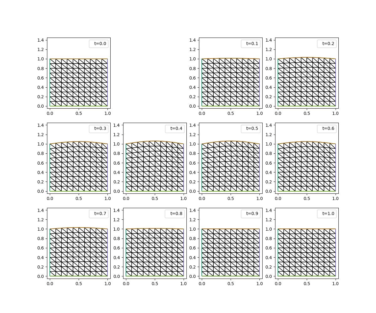
Again, the mesh is deformed according to the vertical displacement on the top boundary, with the left, right, and bottom boundaries remaining fixed, returning to be very close to its original state after one period. Let’s check this in the ${\ell }_{\mathrm{\infty }}$ norm.

coord_data = mover.mesh.coordinates.dat.data
linf_error = np.max(np.abs(coord_data - coord_data_init))
print(f"l_infinity error: {linf_error:.3f} m")
assert linf_error < 0.002

l_infinity error: 0.001 m

Note that the mesh doesn’t return to its original state quite as neatly with the lineal spring method as it does with the Laplacian smoothing method. However, the result is still very good (as can be seen from the plots above).

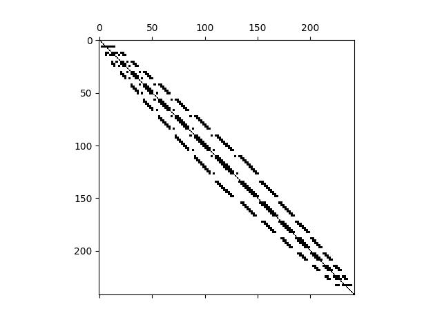
We can view the sparsity pattern of the stiffness matrix as follows.

K = mover.assemble_stiffness_matrix(boundary_conditions=boundary_conditions)
print(f"Stiffness matrix shape: {K.shape}")
print(f"Number of mesh vertices: {mesh.num_vertices()}")

Stiffness matrix shape: (242, 242)
Number of mesh vertices: 121

fig, axes = plt.subplots()
axes.spy(K)
plt.savefig("lineal_spring-sparsity.jpg")

This tutorial can be dowloaded as a Python script.

References

[FDKL98]

Charbel Farhat, Christoph Degand, Bruno Koobus, and Michel Lesoinne. Torsional springs for two-dimensional dynamic unstructured fluid meshes. Computer methods in applied mechanics and engineering, 163(1-4):231–245, 1998.