Steady-state adaptation (Poisson equation)

In this demo we introduce fundamental ideas of anisotropic mesh adaptation and demonstrate how Animate allows us to fine-tune the mesh adaptation process. We consider the steady-state Poisson equation described in [Dundovic et al., 2024]. The Poisson equation is solved on a unit square domain with homogeneous Dirichlet boundary conditions. Using the method of manufactured solutions, the function \(u(x,y) = (1-e^{-x/\epsilon})(x-1)\sin(\pi y)\), where \(\epsilon=0.01\), is selected as the exact solution, with the corresponding Poisson equation given by

\[\nabla^2 u = \left( \left(2/\epsilon - 1/\epsilon^2\right) e^{-x/\epsilon} - \pi^2 (x-1)\left(1 - e^{-x/\epsilon}\right) \right) \sin(\pi y).\]

Let us plot the exact solution.

import matplotlib.pyplot as plt
from firedrake import *
from firedrake.pyplot import *

epsilon = Constant(0.01)

uniform_mesh = UnitSquareMesh(64, 64)
x, y = SpatialCoordinate(uniform_mesh)
V = FunctionSpace(uniform_mesh, "CG", 2)
u_exact = Function(V).interpolate((1 - exp(-x / epsilon)) * (x - 1) * sin(pi * y))

fig, ax = plt.subplots()
# tripcolor(u_exact, axes=ax, shading="flat")
im = tricontourf(u_exact, axes=ax, cmap="coolwarm", levels=20)
ax.set_xlim(0, 1)
ax.set_ylim(0, 1)
ax.set_aspect("equal")
fig.colorbar(im, ax=ax)
fig.savefig("poisson_exact-solution.jpg", bbox_inches="tight")

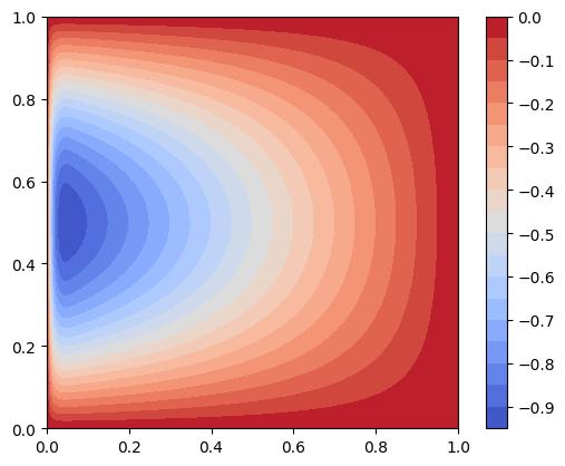
We observe that the solution exhibits a sharp gradient in the \(x\)-direction near the \(x=0\) boundary since the term \(1-e^{-x/\epsilon}\) decays rapidly. Since the solution exhibits less rapid variation in the \(y\)-direction compared to the \(x\)-direction, we expect anisotropic mesh adaptation to be beneficial. Let’s test this.

First, define a function that solves the Poisson equation on a given mesh.

def solve_poisson(mesh):
    V = FunctionSpace(mesh, "CG", 2)
    x, y = SpatialCoordinate(mesh)
    f = Function(V)

    eps = 0.01
    f.interpolate(
        -sin(pi * y)
        * ((2 / eps) * exp(-x / eps) - (1 / eps**2) * (x - 1) * exp(-x / eps))
        + pi**2 * sin(pi * y) * ((x - 1) - (x - 1) * exp(-x / eps))
    )

    u = TrialFunction(V)
    v = TestFunction(V)

    a = inner(grad(u), grad(v)) * dx
    L = f * v * dx

    bcs = [DirichletBC(V, Constant(0.0), "on_boundary")]

    u_numerical = Function(V)
    solve(a == L, u_numerical, bcs=bcs)

    return u_numerical

Now we can solve the Poisson equation on the above-defined uniform mesh. We will also compute the error between the numerical solution and the exact solution.

u_numerical = solve_poisson(uniform_mesh)
error = errornorm(u_numerical, u_exact)
print(f"Error on uniform mesh = {error:.2e}")
print(f"Number of elements = {uniform_mesh.num_cells()}")

Error on uniform mesh = 1.50e-03
Number of elements = 8192

In previous demos we have seen how to adapt a mesh using a RiemannianMetric object, where we defined the metric from analytical expressions. Such approaches may be suitable for problems in which we know beforehand where fine resolution is required and where coarse resolution is acceptable. A more general approach is to adapt the mesh based on the features of the solution field; i.e., based on its Hessian. Animate provides several Hessian recovery methods through the animate.metric.RiemannianMetric.compute_hessian() method.

For example, we compute the Hessian of the above numerical solution as follows.

from animate.metric import RiemannianMetric

P1_ten = TensorFunctionSpace(uniform_mesh, "CG", 1)
isotropic_metric = RiemannianMetric(P1_ten)
isotropic_metric.compute_hessian(u_numerical)

Before adapting the mesh from the metric above, let us further modify the metric. We can do this using the set_parameters() method. We must always specify the target complexity, which will influence the number of elements in the adapted mesh (i.e., the higher the target complexity, the more elements in the adapted mesh). We can specify many other parameters, such as the maximum tolerated anisotropy. For example, setting the maximum tolerated anisotropy to 1 will yield an isotropic metric.

isotropic_metric_parameters = {
    "dm_plex_metric_target_complexity": 200,
    "dm_plex_metric_a_max": 1,
}
isotropic_metric.set_parameters(isotropic_metric_parameters)
isotropic_metric.normalise()

Note that these parameters are not guaranteed to be satisfied exactly. They certainly will not be in this case, since it is impossible to tesselate a rectangular domain with non-overlapping equilateral triangles.

To analyse the metric, it is useful to visualise its density and anisotropy quotient components (see the documentation).

def plot_metric(metric, figname):
    density, quotients, _ = metric.density_and_quotients()

    fig, axes = plt.subplots(1, 2, sharex=True, sharey=True)
    im_density = tripcolor(density, axes=axes[0], norm="log", cmap="coolwarm")
    # Plot the first anisotropy quotient, which is the reciprocal of the second quotient
    im_quotients = tripcolor(
        quotients.sub(0), axes=axes[1], norm="log", cmap="coolwarm"
    )
    axes[0].set_title("Metric density")
    axes[1].set_title("Metric anisotropy quotient")
    for ax in axes:
        ax.set_xlim(0, 1)
        ax.set_ylim(0, 1)
        ax.set_aspect("equal")
    fig.colorbar(im_density, ax=axes[0], orientation="horizontal")
    cbar_q = fig.colorbar(im_quotients, ax=axes[1], orientation="horizontal")
    cbar_q.ax.tick_params(which="minor", labelbottom=False)
    fig.savefig(figname, bbox_inches="tight")


plot_metric(isotropic_metric, "poisson_isotropic-metric.jpg")

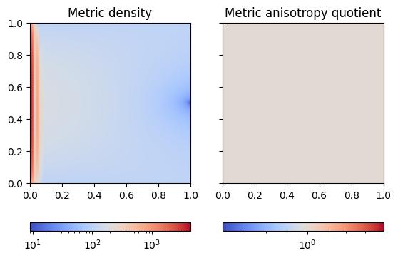
We observe that the metric density is multiple orders of magnitude larger near the \(x=0\) boundary compared to the rest of the domain. In comparison, the anisotropy quotient is equal to unity throughout the domain.

Finally, let us adapt the original uniform mesh from the above-defined metric.

from animate.adapt import adapt

isotropic_mesh = adapt(uniform_mesh, isotropic_metric)

fig, axes = plt.subplots(1, 2)
triplot(isotropic_mesh, axes=axes[0])
triplot(isotropic_mesh, axes=axes[1])
axes[0].set_xlim(0, 1)
axes[0].set_ylim(0, 1)
axes[1].set_xlim(0, 0.15)
axes[1].set_ylim(0.4, 0.6)
for ax in axes:
    ax.set_aspect("equal")
fig.suptitle("Isotropic mesh")
fig.tight_layout()
fig.savefig("poisson_isotropic-mesh.jpg", bbox_inches="tight")

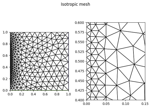
As expected, the adapted mesh is isotropic, with the finest local resolution near the \(x=0\) boundary. The size of the elements is gradually increasing away from the boundary, at a maximum factor determined by the dm_plex_metric_gradation_factor parameter. The default value is 1.3, which means that adjacent element edge lengths cannot differ by more than a factor of 1.3.

Let us again solve the Poisson equation, but now on the isotropic adapted mesh.

u_numerical_isotropic = solve_poisson(isotropic_mesh)
V_isotropic = FunctionSpace(isotropic_mesh, "CG", 2)
u_exact_isotropic = Function(V_isotropic).interpolate(u_exact)
error = errornorm(u_numerical_isotropic, u_exact_isotropic)
print(f"Error on isotropic mesh = {error:.2e}")
print(f"Number of elements = {isotropic_mesh.num_cells()}")

Error on isotropic mesh = 9.61e-04
Number of elements = 2987

We have achieved similar accuracy compared to the uniform mesh, but with almost three times fewer elements.

Let us repeat the above process, but this time using an anisotropic metric; i.e., we use the default maximum tolerated anisotropy value of \(10^5\).

anisotropic_metric = RiemannianMetric(P1_ten)
anisotropic_metric_parameters = {
    "dm_plex_metric_target_complexity": 200,
}
anisotropic_metric.set_parameters(anisotropic_metric_parameters)
anisotropic_metric.compute_hessian(u_numerical)
anisotropic_metric.normalise()

plot_metric(anisotropic_metric, "poisson_anisotropic-metric.jpg")

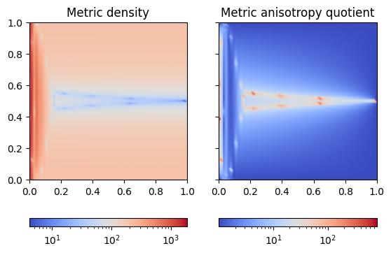
While the metric density field is similar to that of the isotropic metric, we now observe a variation in the anisotropy quotient throughout the domain. The region near the \(x=0\) boundary and a region around \(y=0.5\) have a high anisotropy quotient of more than 30 (in some parts over 100), while the rest of the domain remains isotropic. Recall that the metric will again be smoothened through the metric gradation process.

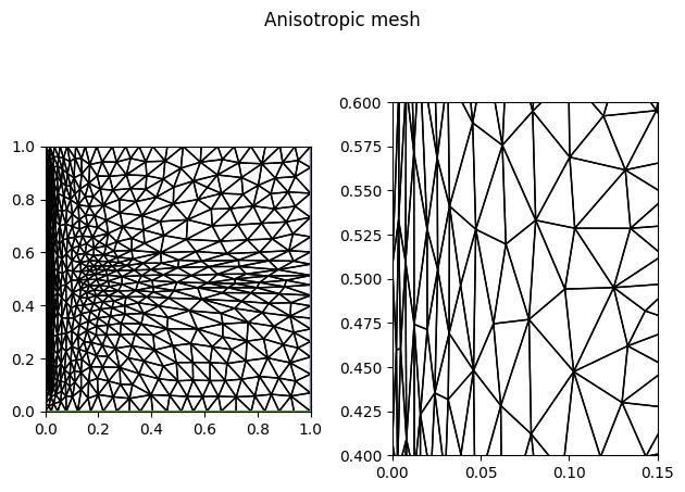
Let’s adapt the mesh again and compare it to the isotropic one.

anisotropic_mesh = adapt(uniform_mesh, anisotropic_metric)

fig, axes = plt.subplots(1, 2)
triplot(anisotropic_mesh, axes=axes[0])
triplot(anisotropic_mesh, axes=axes[1])
axes[0].set_xlim(0, 1)
axes[0].set_ylim(0, 1)
axes[1].set_xlim(0, 0.15)
axes[1].set_ylim(0.4, 0.6)
for ax in axes:
    ax.set_aspect("equal")
fig.suptitle("Anisotropic mesh")
fig.tight_layout()
fig.savefig("poisson_anisotropic-mesh.jpg", bbox_inches="tight")

u_numerical_anisotropic = solve_poisson(anisotropic_mesh)
u_exact_anisotropic = Function(FunctionSpace(anisotropic_mesh, "CG", 2))
u_exact_anisotropic.interpolate(u_exact)
error = errornorm(u_numerical_anisotropic, u_exact_anisotropic)
print(f"Error on anisotropic mesh = {error:.2e}")
print(f"Number of elements = {anisotropic_mesh.num_cells()}")

Error on anisotropic mesh = 9.53e-04
Number of elements = 964

We have again achieved similar accuracy compared to the uniform and isotropic meshes, but with eight and three times fewer elements, respectively. The largest difference in local resolution is near the \(x=0\) boundary, where the elements of the anisotropic mesh are elongated in the \(y\)-direction. Since the solution accuracy remained similar, we can conclude that the additional refinement in the \(x\)-direction in the isotropic case was not beneficial.

Exercise

Experiment with different metric parameters and their values. For example, try changing the metric gradation factor mentioned above, or the minimum and maximum tolerated metric magnitude (dm_plex_metric_h_min and dm_plex_metric_h_max, respectively).

This demo can also be accessed as a Python script.