Intersecting and averaging metric fields

As we saw in the previous demo, the metric tells the mesh adaptivity library what the desired edge lengths is in different directions, in different parts of the domain. As we will see these desired edge lengths are often based on an estimate of the discretisation error we want to minimize for a certain solution field. Therefore, if in a model we are solving for multiple fields, we may end up with multiple metric fields telling us about the desired edge lengths for the discretisation of each of these fields individually. If we want the model to employ a single optimal mesh for the discretisation of all of these fields however, we need a way to combine the metrics taking into account the different requirements for the different solution fields. The same functionality is needed if in a time-dependent model we have multiple metrics based on the solution at different timesteps, and we want to adapt the mesh optimally for all of these timesteps combined.

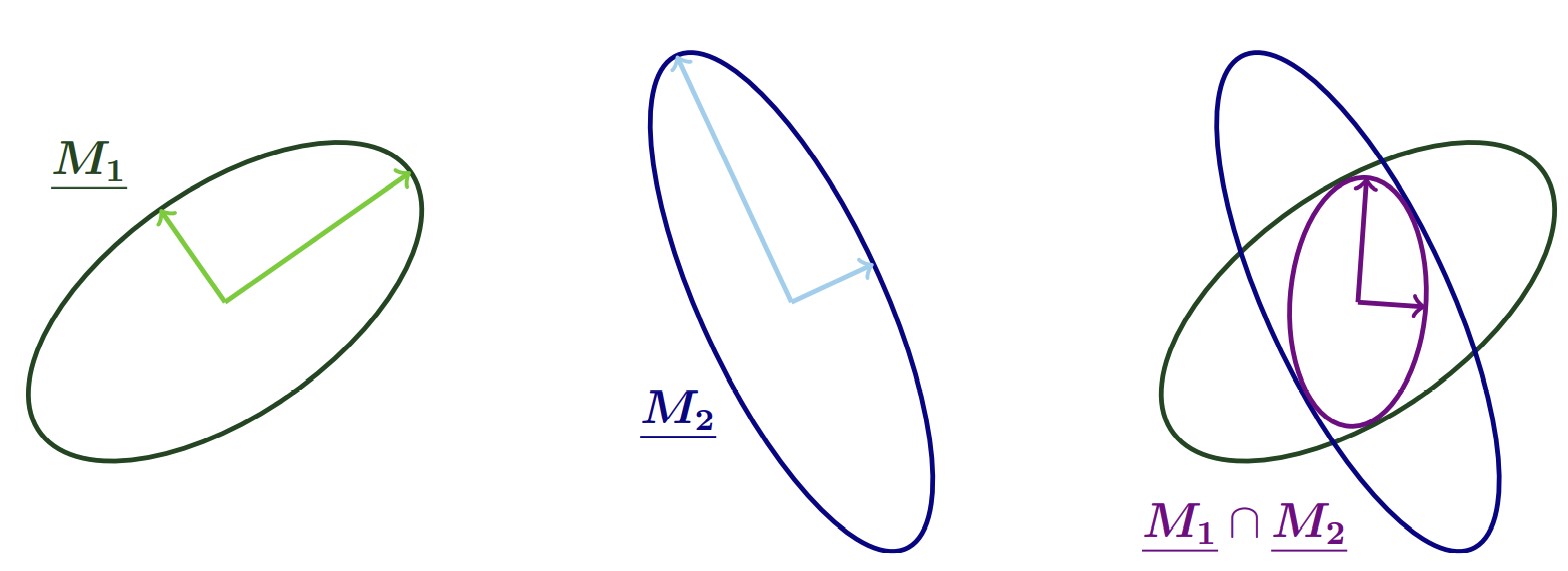
A natural way to combine two metrics for mesh adaptation, is the so called intersection method. A natural, geometric interpretation exists if we represent the individual metrics by ellipsoids, which indicate the desired edge length in different directions through their principle axes. The intersection of two metrics produces a metric whose associated ellipsoid is the largest ellipsoid that can fit within the ellipsoids of the two metrics:

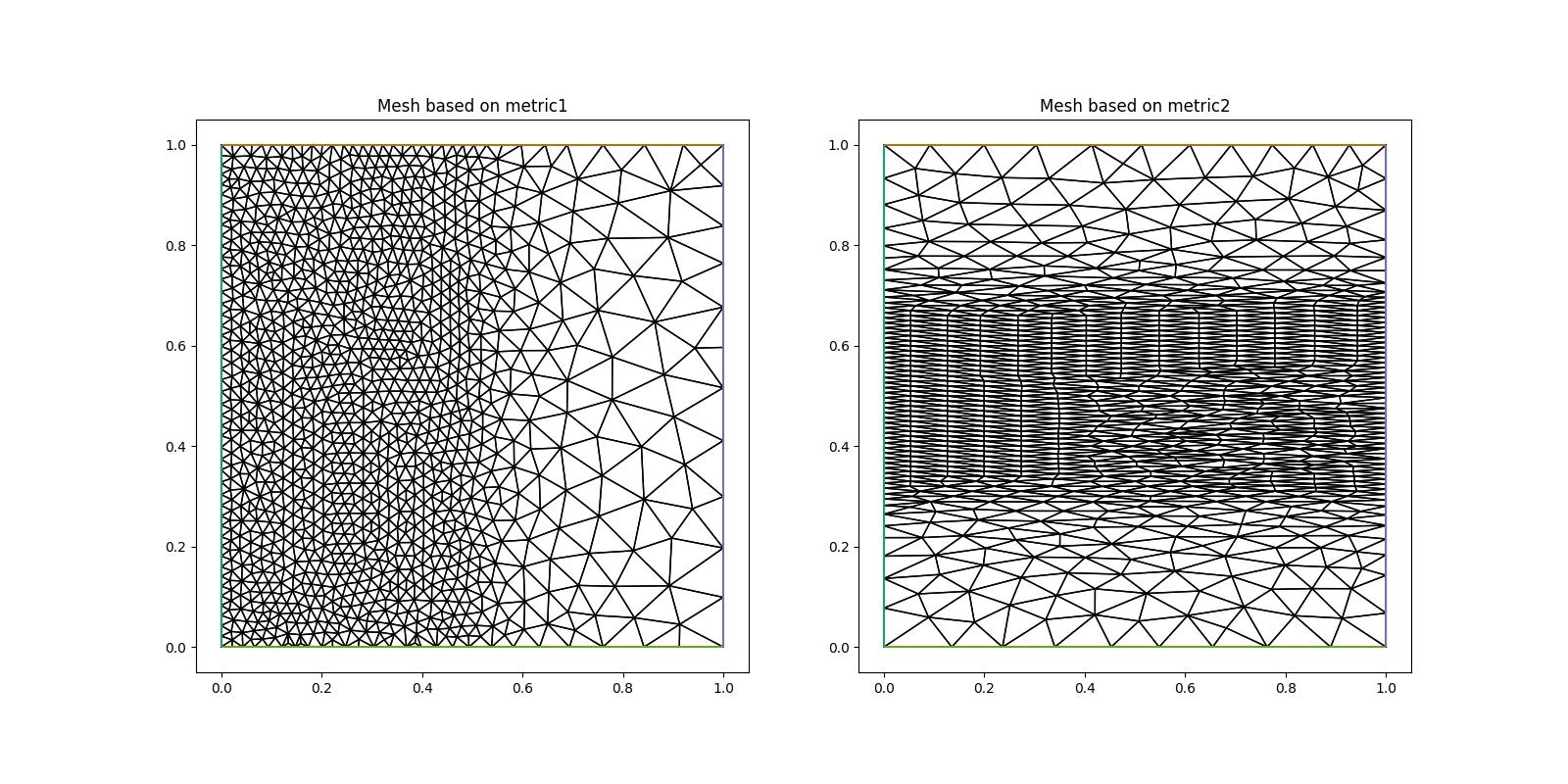
Below we first set up two metrics: Metric 1 asks for a medium resolution of \(hm=0.025\) in the left, and a coarse resolution of \(hc=0.1\) in the right half of the domain. Metric 2 prescribes the coarse resolution for \(y<0.3\) and \(y>0.7\), but asks for an anisotropic resolution, \(hc\) in the \(x\)-direction and \(hf=0.01\) in the \(y\)-direction, for \(0.3<y<0.7\)

import matplotlib.pyplot as plt
from firedrake import *
from firedrake.pyplot import triplot

from animate import *

mesh = UnitSquareMesh(100, 100)
P1_ten = TensorFunctionSpace(mesh, "CG", 1)
metric1 = RiemannianMetric(P1_ten)
metric2 = RiemannianMetric(P1_ten)
x, y = SpatialCoordinate(mesh)
r = 0.2
hf = 0.01
hm = 0.025
hc = 0.1
anisotropic = as_matrix([[1 / hc**2, 0], [0, 1 / hf**2]])
medium = as_matrix([[1 / hm**2, 0], [0, 1 / hm**2]])
coarse = as_matrix([[1 / hc**2, 0], [0, 1 / hc**2]])
metric1.interpolate(conditional(x < 0.5, medium, coarse))
metric2.interpolate(
    conditional(And(abs(x - 0.5) < r, abs(y - 0.5) < r), anisotropic, coarse)
)
metric2.interpolate(conditional(abs(y - 0.5) < r, anisotropic, coarse))
mesh1 = adapt(mesh, metric1)
mesh2 = adapt(mesh, metric2)
fig, axes = plt.subplots(figsize=(16, 8), ncols=2)
triplot(mesh1, axes=axes[0])
axes[0].set_aspect("equal")
axes[0].set_title("Mesh based on metric1")
triplot(mesh2, axes=axes[1])
axes[1].set_aspect("equal")
axes[1].set_title("Mesh based on metric2")
fig.show()
fig.savefig("combining_metrics-inputs.jpg")

We can intersect multiple metric by using the intersect() method of a RiemannianMetric, which intersects the given metric with another, or multiple, provided metrics. We therefore first make a copy of metric1 and then intersect it with metric2:

intersected_metric = metric1.copy(deepcopy=True)
intersected_metric.intersect(metric2)
mesh_intersected = adapt(mesh, intersected_metric)
fig, axes = plt.subplots(figsize=(16, 16))
triplot(mesh_intersected, axes=axes)
axes.set_aspect("equal")
axes.set_title("Mesh based on intersected metric")
fig.show()
fig.savefig("combining_metrics-intersection.jpg")

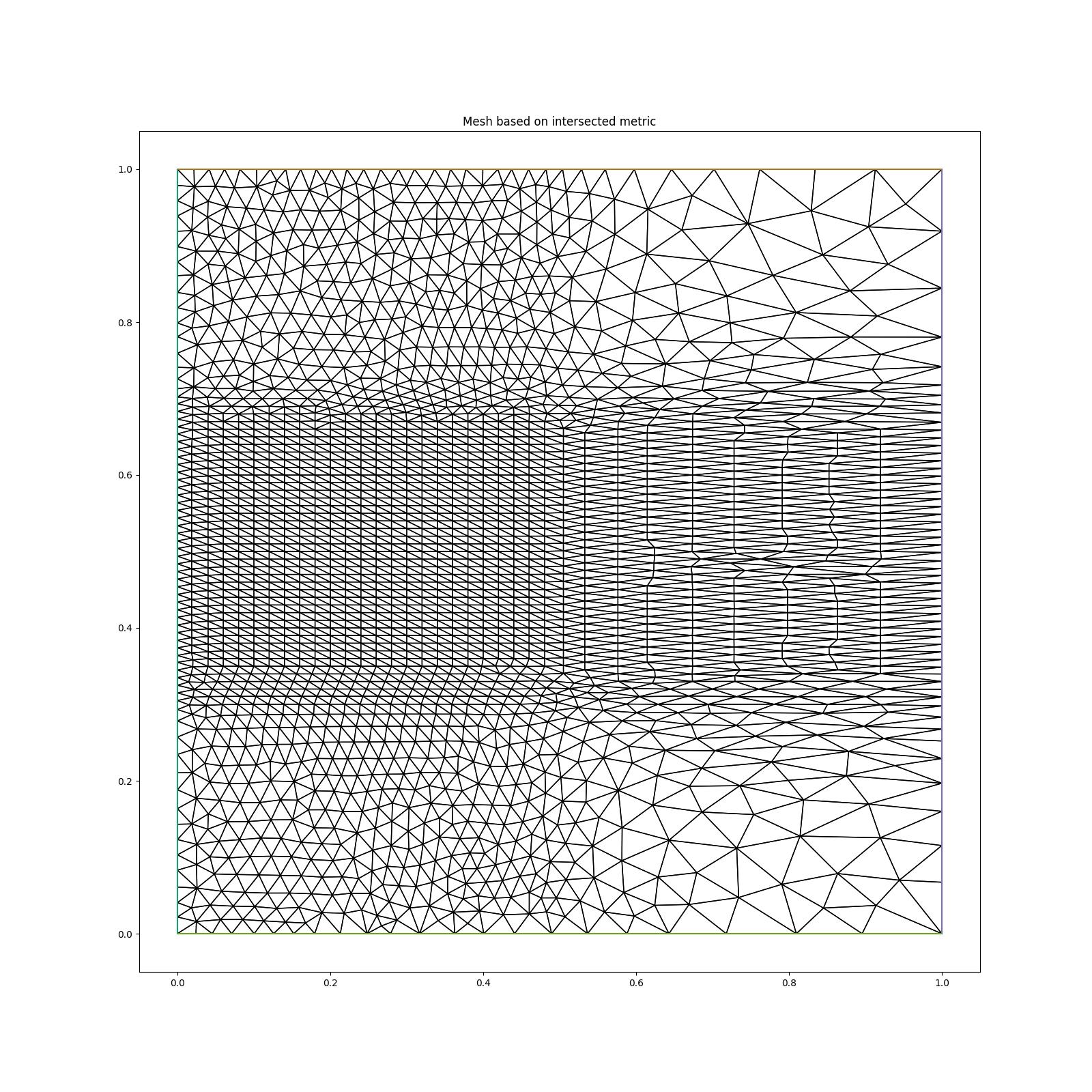
As we can observe, in every region the resolution respects the minimum resolution in all directions asked for by both metrics. For example, in the region \(x<0.5\), \(0.3<y<0.7\) the resolution in the \(x\)-direction is \(hf=0.01\), as required by metric2, but in the \(y\)-direction the resolution is \(hm=0.02\) as required by metric1.

If instead we average the metrics using the average() method,

averaged_metric = metric1.copy(deepcopy=True)
averaged_metric.average(metric2)
mesh_averaged = adapt(mesh, averaged_metric)
fig, axes = plt.subplots(figsize=(16, 16))
triplot(mesh_averaged, axes=axes)
axes.set_aspect("equal")
axes.set_title("Mesh based on averaged metric")
fig.show()
fig.savefig("combining_metrics-averaging.jpg")

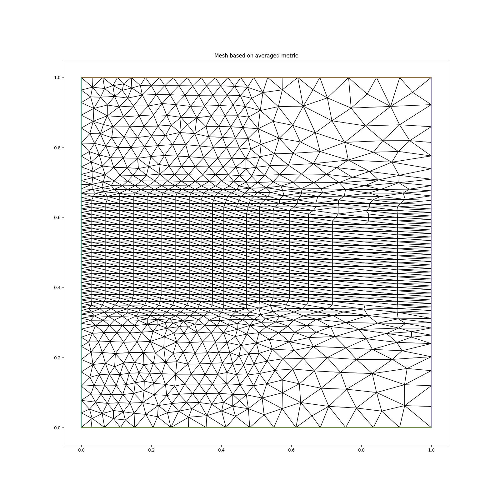
the resolution in, e.g., the region \(x<0.5, y<0.3\) is now based on an average of \(hm=0.02\) and \(hc=0.1\), i.e. an edge length of 0.06.

The next demo will consider a different topic: transferring fields between meshes.

This demo can also be accessed as a Python script.