Object-oriented Burgers equation
You may have noticed that the functions get_form(),
get_solver(), get_initial_condition() and
get_qoi() all take a MeshSeq, AdjointMeshSeq
or GoalOrientedMeshSeq as input and return a function.
If this all feels a lot like writing methods for a
subclass, that’s because this is exactly what we are doing.
The constructors for MeshSeq, AdjointMeshSeq and
GoalOrientedMeshSeq simply take these functions and adopt
them as methods. A more natural way to write the subclass yourself.
In the following, we mostly copy the contents from the previous
demos and combine the methods into a subclass called
BurgersMeshSeq. The main difference to note is that
get_qoi() should get the annotate_qoi() decorator
so that it gets modified internally to account for annotation.
from firedrake import *

from goalie import *

set_log_level(DEBUG)


class BurgersMeshSeq(GoalOrientedMeshSeq):
    def get_initial_condition(self):
        fs = self.function_spaces["u"][0]
        x, y = SpatialCoordinate(self[0])
        return {"u": Function(fs).interpolate(as_vector([sin(pi * x), 0]))}

    def get_solver(self):
        def solver(index):
            u, u_ = self.field_functions["u"]

            # Define constants
            R = FunctionSpace(self[index], "R", 0)
            dt = Function(R).assign(self.time_partition.timesteps[index])
            nu = Function(R).assign(0.0001)

            # Setup variational problem
            v = TestFunction(u.function_space())
            F = (
                inner((u - u_) / dt, v) * dx
                + inner(dot(u, nabla_grad(u)), v) * dx
                + nu * inner(grad(u), grad(v)) * dx
            )

            # Communicate variational form to mesh_seq
            self.read_forms({"u": F})

            # Time integrate from t_start to t_end
            t_start, t_end = self.subintervals[index]
            dt = self.time_partition.timesteps[index]
            t = t_start
            qoi = self.get_qoi(index)
            while t < t_end - 1.0e-05:
                solve(F == 0, u, ad_block_tag="u")
                if self.qoi_type == "time_integrated":
                    self.J += qoi(t)
                yield

                u_.assign(u)
                t += dt

        return solver

    @annotate_qoi
    def get_qoi(self, i):
        R = FunctionSpace(self[i], "R", 0)
        dt = Function(R).assign(self.time_partition.timesteps[i])

        def end_time_qoi():
            u = self.field_functions["u"][0]
            return inner(u, u) * ds(2)

        def time_integrated_qoi(t):
            u = self.field_functions["u"][0]
            return dt * inner(u, u) * ds(2)

        if self.qoi_type == "end_time":
            return end_time_qoi
        else:
            return time_integrated_qoi
Notice that the get_solver() and get_qoi_function()
methods have been modified to account for both "end_time" and
"time_integrated" QoIs.
We apply exactly the same setup as before, except that the BurgersMeshSeq
class is used and we again need to specifically define the mesh for each subinterval.
n = 32
meshes = [UnitSquareMesh(n, n), UnitSquareMesh(n, n)]
fields = [Field("u", family="Lagrange", degree=2, vector=True)]

end_time = 0.5
dt = 1 / n
num_subintervals = len(meshes)
time_partition = TimePartition(
    end_time, num_subintervals, dt, fields, num_timesteps_per_export=2
)
mesh_seq = BurgersMeshSeq(time_partition, meshes, qoi_type="time_integrated")
solutions, indicators = mesh_seq.indicate_errors(
    enrichment_kwargs={"enrichment_method": "h"}
)
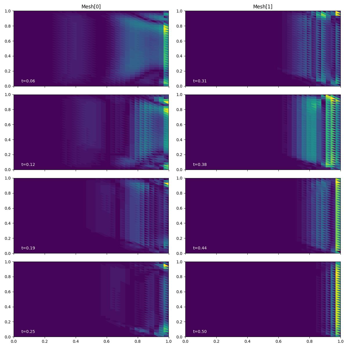
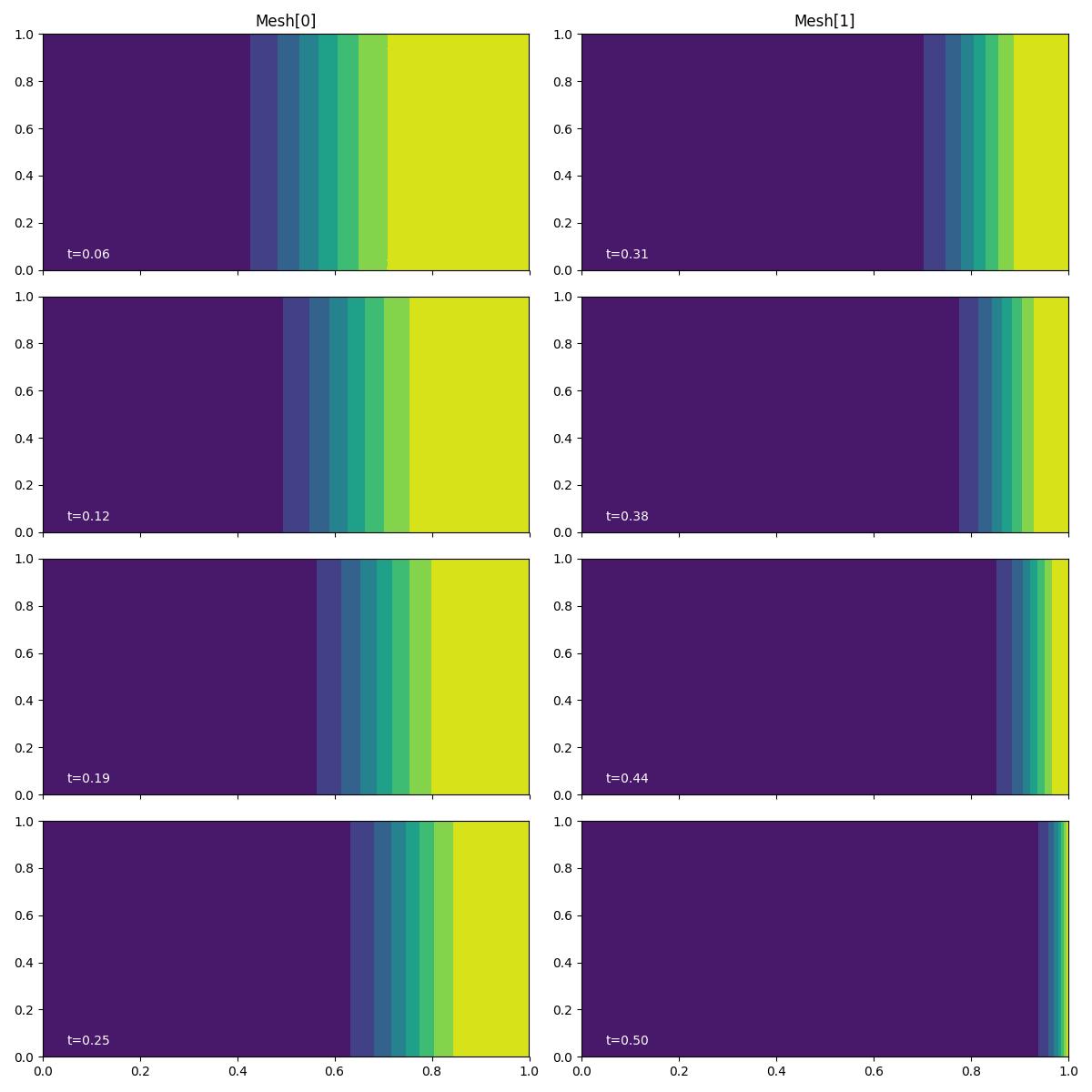
Plotting this, we find that the results are consistent with those generated previously.
fig, axes, tcs = plot_indicator_snapshots(indicators, time_partition, "u", levels=50)
fig.savefig("burgers-oo_ee.jpg")

fig, axes, tcs = plot_snapshots(solutions, time_partition, "u", "adjoint")
fig.savefig("burgers-oo-time_integrated.jpg")

In the next demo, we move on from Burgers equation to consider a linear advection example with a rotational velocity field.
This demo can also be accessed as a Python script.